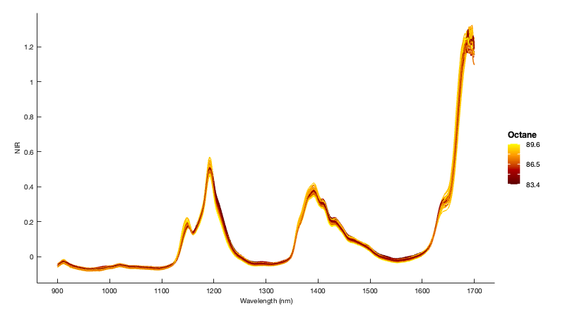
gramm data visualization toolbox
편집자 메모: This file was selected as MATLAB Central Pick of the Week
Gramm is a powerful plotting toolbox which allows to quickly create complex, publication-quality figures in MATLAB, and is inspired by R's ggplot2 library by Hadley Wickham. As a reference to this inspiration, gramm stands for GRAMmar of graphics for MATLAB.
Gramm is a data visualization toolbox for MATLAB that allows to produce publication-quality plots from grouped data easily and flexibly. MATLAB can be used for complex data analysis using a high-level interface: it supports mixed-type tabular data via tables, provides statistical functions that accept these tables as arguments, and allows users to adopt a split-apply-combine approach (Wickham 2011) with rowfun(). However, the standard plotting functionality in MATLAB is mostly low-level, allowing to create axes in figure windows and draw geometric primitives (lines, points, patches) or simple statistical visualizations (histograms, boxplots) from numerical array data. Producing complex plots from grouped data thus requires iterating over the various groups in order to make successive statistical computations and low-level draw calls, all the while handling axis and color generation in order to visually separate data by groups. The corresponding code is often long, not easily reusable, and makes exploring alternative plot designs tedious.
Inspired by ggplot2 (Wickham 2009), the R implementation of "grammar of graphics" principles (Wilkinson 1999), gramm improves MATLAB's plotting functionality, allowing to generate complex figures using high-level object-oriented code. Gramm has been used in several publications in the field of neuroscience, from human psychophysics (Morel et al. 2017), to electrophysiology (Morel et al. 2016; Ferrea et al. 2017), human functional imaging (Wan et al. 2017) and animal training (Berger et al. 2017).
- Automatically within MATLAB : Open the Add-ons explorer, search for "gramm" and click Add !
- Or by townloading the toolbox package : download the latest .mltbx file from the GitHub Releases and double-click the downloaded file to install.
- Or manually : download the gramm toolbox from the MATLAB File exchange or GitHub ("Clone or download" button>download ZIP) or clone it, and add the folder containing the @gramm class folder to your MATLAB path (using the GUI or
addpath())
- gramm cheat sheet
- Numerous coding examples and test cases in
examples.m, exported for preview in html/examples.html - From MATLAB:
doc grammto find links to the documentation of each method.
Gramm has been published in the Journal of Open Source Software. If you use gramm plots in a publication you can thus cite it using the following:
Morel, (2018). Gramm: grammar of graphics plotting in Matlab. Journal of Open Source Software, 3(23), 568, https://doi.org/10.21105/joss.00568
Tested under MATLAB 2014b+ versions. With pre-2014b versions, gramm forces 'painters', renderer to avoid some graphic bugs, which deactivates transparencies (use non-transparent geoms, for example stat_summary('geom','lines')). The statistics toolbox is required for some methods: stat_glm(), some stat_summary() methods, stat_density(). The curve fitting toolbox is required for stat_fit().
The typical workflow to generate a figure with gramm is the following:
- In a first step, provide gramm with the relevant data for the figure: X and Y variables, but also grouping variables that will determine color, subplot rows/columns, etc.
- In the next steps, add graphical layers to your figure: raw data layers (directly plot data as points, lines...) or statistical layers (plot fits, histograms, densities, summaries with confidence intervals...). One instruction is enough to add each layer, and all layers offer many customization options.
- In the last step, gramm draws the figure, and takes care of all the annoying parts: no need to loop over colors or subplots, colors and legends are generated automatically, axes limits are taken care of, etc.
For example, with gramm, 7 lines of code are enough to create the figure below from the carbig dataset. Here the figure represents the evolution of fuel economy of new cars in time, with number of cylinders indicated by color, and regions of origin separated across subplot columns:
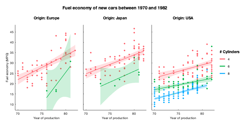
load carbig.mat %Load example dataset about cars
origin_region=num2cell(org,2); %Convert origin data to a cellstr

% Create a gramm object, provide x (year of production) and y (fuel economy) data,
% color grouping data (number of cylinders) and select a subset of the data
g=gramm('x',Model_Year,'y',MPG,'color',Cylinders,'subset',Cylinders~=3 & Cylinders~=5)
% Subdivide the data in subplots horizontally by region of origin
g.facet_grid([],origin_region)
% Plot raw data as points
g.geom_point()
% Plot linear fits of the data with associated confidence intervals
g.stat_glm()
% Set appropriate names for legends
g.set_names('column','Origin','x','Year of production','y','Fuel economy (MPG)','color','# Cylinders')
%Set figure title
g.set_title('Fuel economy of new cars between 1970 and 1982')
% Do the actual drawing
g.draw()To export figures in a vector-based format, use the SVG or PDF option rather than EPS. SVG can be read by all vector editing softwares and causes less problems than EPS both for export and import (transparency support, text without cuts, etc.). gramm has a convenient export() method that can be called after draw() and maintains correct dimensions/aspect ratio.
-
Accepts X Y and Z data as arrays, matrices or cells of arrays
-
Accepts grouping data as arrays or cellstr.
-
Multiple ways of separating groups of data:
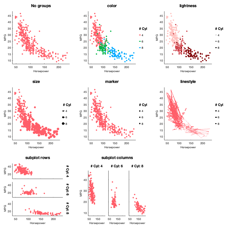
- Colors, lightness, point markers, line styles, and point/line size (
'color','lightness','marker','linestyle','size') - Subplots by row and/or columns, or wrapping columns (
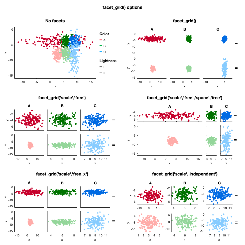
facet_grid()andfacet_wrap()). Multiple options for consistent axis limits across facets, rows, columns, etc. (using'scale'and'space') - Separate figures (
fig())
- Colors, lightness, point markers, line styles, and point/line size (
-
Multiple ways of directly plotting the data:
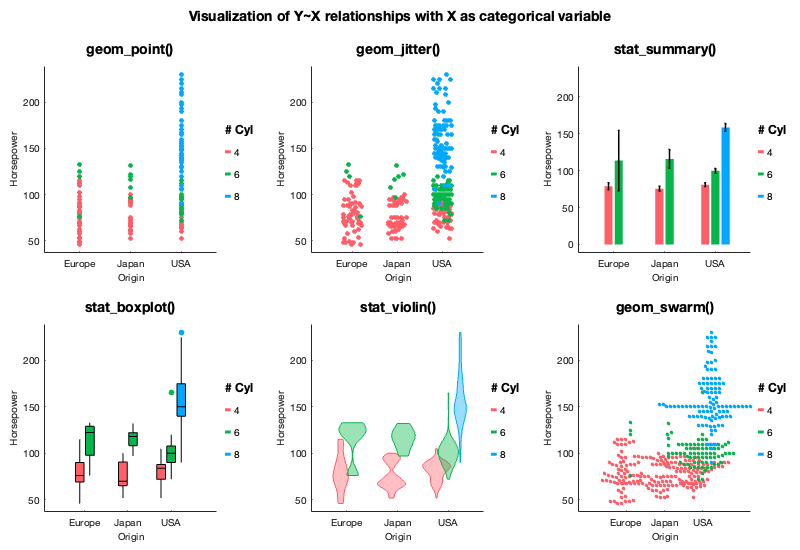
- scatter plots (
geom_point()) and jittered scatter plot (geom_jitter()) - lines (
geom_line()) - pre-computed confidence intervals (
geom_interval()) - bars plots (
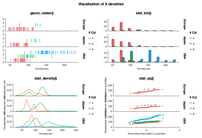
geom_bar()) - raster plots (
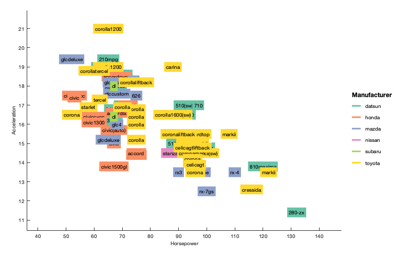
geom_raster()) - labels (
geom_label()) - point counts (
geom_count()) - swarm / beeswarm plots (
geom_swarm())
- scatter plots (
-
Multiple ways of plotting statistics on the data:
- y data summarized by x values (uniques or binned) with confidence intervals (
stat_summary()) - histograms and density plots of x values (
stat_bin()andstat_density()) - box and whisker plots (
stat_boxplot()) - violin plots (
stat_violin()) - quantile-quantile plots (
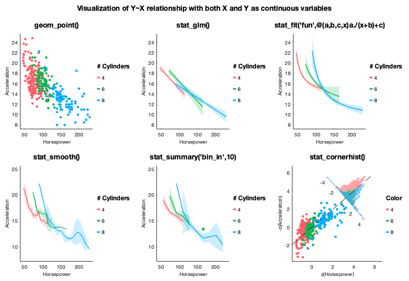
stat_qq()) of x data distribution against theoretical distribution or y data distribution. - spline-smoothed y data with optional confidence interval (
stat_smooth()) - 2D binning (
stat_bin2d()) - GLM fits (
stat_glm(), requires statistics toolbox) - Custom fits with user-provided anonymous function (
stat_fit()) - Ellipses of confidence (
stat_ellipse())
- y data summarized by x values (uniques or binned) with confidence intervals (
-
When Z data is provided in the call to
gramm(),geom_point(),geom_line()andgeom_label()generate 3D plots -
Subplots are created without too much empty space in between (and resize properly !)
-
Polar coordinates (
set_polar()) -
Color data can also be displayed as a continous variable, not as a grouping factor (
set_continuous_color()) -
X and Y axes can be flipped to get horizontal statistics visualizations (
coord_flip()) -
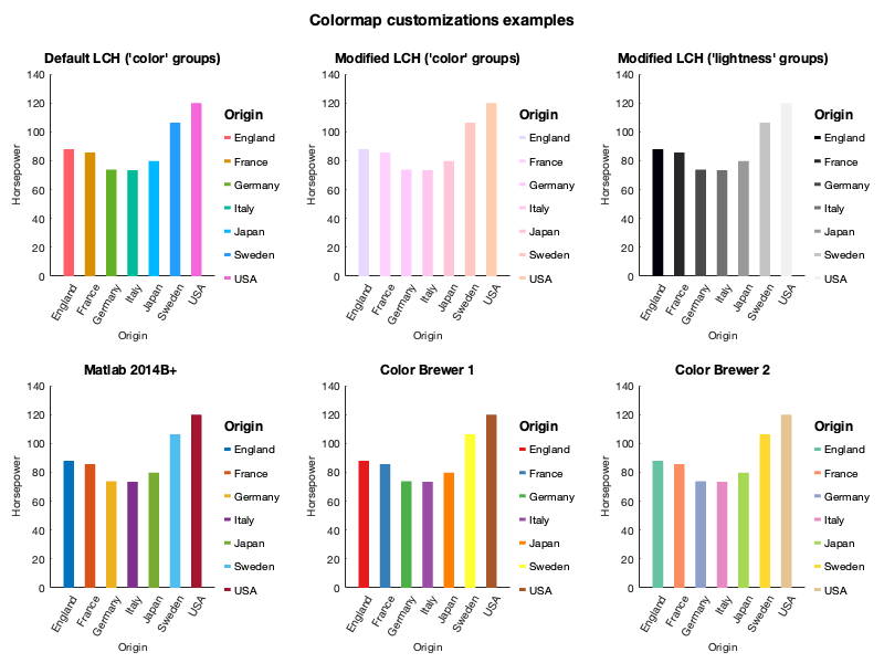
Color generation can be customized in the LCH color space, or can use alternative colormaps (MATLAB's default, colorbrewer2), or provide a custom colormap (
set_color_options()) -
Marker shapes and sizes can be customized with
set_point_options() -
Line styles and width can be customized with
set_line_options() -
Text elements aspect can be customized with
set_text_options() -
Parameters of
stat_functions (alpha level, N bootstraps) can be modified withset_stat_options() -
The ordering of grouping variables can be changed between native, sorted, or custom (
set_order_options) -
Confidence intervals as shaded areas, error bars or thin lines
-
Set the width and dodging of graphical elements in
geom_functions,stat_bin(),stat_summary(), andstat_boxplot(), with'width'and'dodge'arguments -
The member structure
resultscontains the results of computations fromstat_plots as well as graphic handles for all plotted elements -
Figure title (
set_title()) -
Multiple gramm plots can be combined in the same figure by creating a matrix of gramm objects and calling the
draw()method on the whole matrix. An overarching title can be added by callingset_title()on the whole matrix. -
Different groupings can be used for different
stat_andgeom_layers with theupdate()method -
MATLABs axes properties are acessible through the method
axe_property() -
Custom legend labels with
set_names() -
Plot reference line on the plots with
geom_abline(),geom_vline(),geom_hline() -
Plot reference polygons on the plots with
geom_polygon() -
Date ticks with
set_datetick() -
Gramm works best with table-like data: separate variables / structure fields / table columns for the variables of interest, with each variable having as many elements as observations.
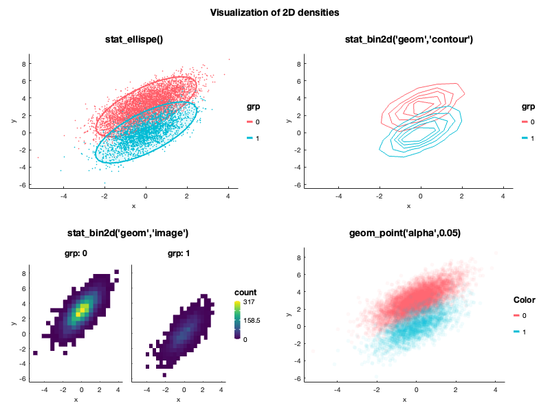
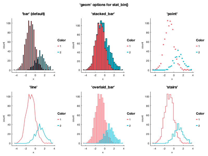
The code for the following figures and many others is in examples.m.
All the mappings presented below can be combined.
Note that we by using Origin as a faceting variable, we visualize exactly the same quantities as in the figure above.
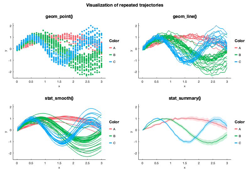
Here the variable given as Y is a Nx1 cell of 1D arrays containing the individual trajectories. Color is given as a Nx1 cellstr.
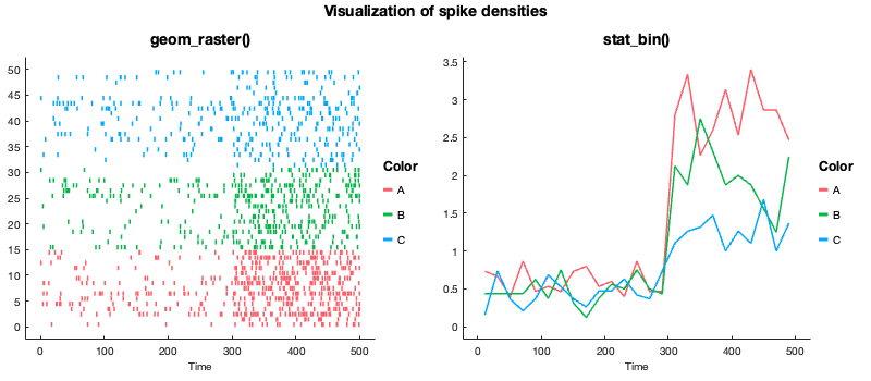
This example highlights the potential use of gramm for neuroscientific data. Here X is a Nx1 cell containing spike trains collected over N trials. Color is given as a Nx1 cellstr.
Using stat_bin() it is possible to construct peristimulus time histograms.
With set_color_options()
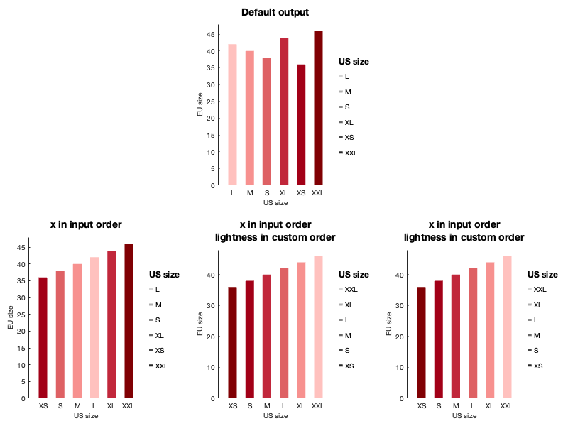
With set_order_options()
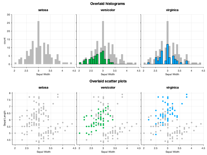
By making calling the update() method after a first draw, the same axes can be reused for another gramm plot. Here this allows to plot the whole dataset in the background of each facet.
gramm was inspired and/or used code from:
- ggplot2
- Panda for color conversion
- subtightplot for subplot creation
- colorbrewer2
- viridis colormap
인용 양식
Morel, Pierre. “Gramm: Grammar of Graphics Plotting in Matlab.” The Journal of Open Source Software, vol. 3, no. 23, The Open Journal, Mar. 2018, p. 568, doi:10.21105/joss.00568.
MATLAB 릴리스 호환 정보
플랫폼 호환성
Windows macOS Linux카테고리
- AI, Data Science, and Statistics > Statistics and Machine Learning Toolbox > ANOVA >
- Sciences > Neuroscience > Frequently-used Algorithms >
- AI, Data Science, and Statistics > Statistics and Machine Learning Toolbox > Descriptive Statistics and Visualization > Statistical Visualization > Box Plots >
태그
Community Treasure Hunt
Find the treasures in MATLAB Central and discover how the community can help you!
Start Hunting!@gramm
@gramm/private
doc
GitHub 디폴트 브랜치를 사용하는 버전은 다운로드할 수 없음
| 버전 | 게시됨 | 릴리스 정보 | |
|---|---|---|---|
| 2.27.1 | See release notes for this release on GitHub: https://github.com/piermorel/gramm/releases/tag/v2.27.1 |
|
|
| 2.27 | See release notes for this release on GitHub: https://github.com/piermorel/gramm/releases/tag/v2.27 |
||
| 2.26 | Switching to new github integration |
|
|
| 2.25 | Added full tab auto-complete for arguments and options with functionSignatures.json |
|
|
| 2.24.2.0 | Updated description |
|
|
| 2.24.0.0 | - Added JOSS paper and DOI information
|
|
|
| 2.23.0.0 | Preparation for JOSS submission |
|
|
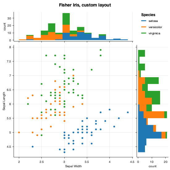
| 2.22.0.0 | Added set_layout_options() allowing to fully customize figure layout in gramm |
||
| 2.21.0.0 | Corrected bug in geom_bar() when used with the 'stacked' option |
|
|
| 2.20.0.0 | - Overhaul of legend and colormap support
|
||
| 2.19.0.0 | Added toggles for row/column labels, improved handling of empty subsets |
|
|
| 2.18.0.0 | - Added more customization options to geom_bar
|
|
|
| 2.17.0.0 | Gramm now merges color and marker/size/linestyle legend if they are the same |
|
|
| 2.16.0.0 | - Added continuous color support to 3D lines and points
|
|
|
| 2.15.0.0 | - Possibility to set ‘CLim’ in set_continuous_color() in order to force color limits.
|
|
|
| 2.14.0.0 | Added geom_polygon() method to add custom polygons on plots |
|
|
| 2.13.0.0 | - Improved graphic fixes for old matlab versions
|
|
|
| 2.12.0.0 | - Added export() method
|
|
|
| 2.11.0.0 | Added coord_flip(), which can be used to generate horizontal box plots, violin plots, error bars, etc. |
|
|
| 2.10.1.0 | - Added the possibility to provide a custom function to stat_summary()
|
|
|
| 2.10.0.0 | - stat_smooth() now provides more smoothing algorithms, better documentation and more conservative CI estimates
|
|
|
| 2.9.0.0 | - Added fig() function to separate data across figures
|
|
|
| 2.8.2.0 | Corrected bug in stat_summary() polar interpolation when x data didn't start at zero radians. Added safety checks. |
|
|
| 2.8.1.0 | - Corrected absence of y ticks if single facet when using facet_wrap()
|
|
|
| 2.8.0.0 | Added 'alpha' option to geom_point(), geom_jitter() and geom_line() |
|
|
| 2.7.0.0 | - Added geom_label() to plot text
|
|
|
| 2.6.0.0 | - Added set_stat_options() to specify alpha level and N bootstrap samples in all stat_ functions
|
|
|
| 2.5.0.0 | Added customization options for text, lines and points:
|
|
|
| 2.4.0.0 | - Added corner histogram of x-y difference stat_cornerhist()
|
||
| 2.3.1.0 | - Added notch option to stat_boxplot()
|
|
|
| 2.3.0.0 | - Added stat_violin() to create violin plots
|
|
|
| 2.2.3.0 | Added functionality to edit legend axes |
|
|
| 2.2.2.0 | - Corrected rare error on y limit computation
|
|
|
| 2.2.1.0 | Corrected error with geom_line() and 3D data |
|
|
| 2.2.0.0 | - Represent user-provided confidence intervals with geom_interval()
|
|
|
| 2.1.1.0 | - Corrected errorbar thickness
|
|
|
| 2.1.0.0 | - Added set_parent() method
|
|
|
| 2.0.1.0 | Updated description |
|
|
| 2.0.0.0 | - Full refactor from a single file to a @gramm class folder
|
|
|
| 1.16.1.0 | Corrected stat_summary() to prevent erroneous line/area interruptions |
|
|
| 1.16.0.0 | - Added 'space' option to facet_grid()
|
|
|
| 1.15.0.0 | - Improved legend layout
|
|
|
| 1.14.1.0 | - Changed Picture |
|
|
| 1.14.0.0 | - ‘z’ input data in gramm() creates 3D plots when using geom_point() or geom_line()
|
|
|
| 1.13.0.0 | Added possibility to set a global title with set_title() |
|
|
| 1.12.2.0 | Description correction |
|
|
| 1.12.1.0 | Added simpler way to set ordering with set_order_options() |
|
|
| 1.12.0.0 | - Added set_order_options()
|
|
|
| 1.11.0.0 | Added box and whiskers plots, Quantile-Quantile plots
|
|
|
| 1.10.0.0 | Added cheat sheet, added geom_funline(), added 'dodge' option to stat_summary() |
|
|
| 1.9.0.0 | - Results from stat_ plots are now returned in the results member structure.
|
|
|
| 1.8.0.0 | Changing manually the limits (using pan or zoom) of a facet in a gramm generated figure will now automatically change the scale of the other facets according to the ‘scale’ facet preferences |
|
|
| 1.7.0.0 | - Added stat_fit() for custom fits (requires curve fitting toolbox)
|
|
|
| 1.6.0.0 | Plenty of new features (separation by lightness, confidence ellipses, color options, geom_hline, geom_vline) |
|
|
| 1.5.1.0 | Bug corrrection |
|
|
| 1.5.0.0 | Enhancements and bug fixes for continuous colors, which can now be forced and customized using set_continuous_color() |
|
|
| 1.4.0.0 | Added ‘edges’ option for custom bins to stat_bin2d() and stat_bin()
|
|
|
| 1.3.0.0 | Greatly improved geom_raster() speed when used with option 'geom','line' |
|
|
| 1.2.0.0 | Additional usage examples |
|
|
| 1.1.0.0 | Corrected set_datetick() issue, corrected initialization of faceting variables |
|
|
| 1.0.0.0 |
|


