Get Started with Audio Signal Processing Using Raspberry Pi
This example shows how to use the Simulink® Support Package for Raspberry Pi® Hardware to get started with audio signal processing applications on the Raspberry Pi hardware. It also shows how to:
Use simulation pacing to slow down a simulation to understand and observe the system behavior. For more information, refer to Simulation Pacing Options.
Use a Spectrum Analyzer and a Time Scope (DSP System Toolbox) to observe and study the audio signals in the frequency and time domains.
Study the significance of sampling frequency and Nyquist criterion.
Prerequisites
For more information on how to use the Simulink Support Package for Raspberry Pi Hardware to run a Simulink model on Raspberry Pi hardware, see Get Started with Simulink Support Package for Raspberry Pi Hardware.
Required Hardware
Raspberry Pi hardware board
USB microphone
Ethernet cable
Mobile phone or any other source of audio that plays the audio in the WAV format
Hardware Setup
In the Hardware Setup dialog box, in the Network Settings screen, select
Connect directly to host computerto avoid any network latency.Connect a USB microphone to the Raspberry Pi hardware board.
Configure Simulink Model and Calibrate Parameters
Open the raspberrypi_audio_gettingStarted Simulink model.
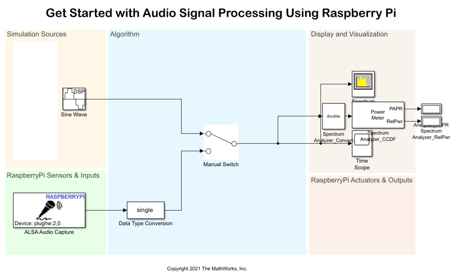
This example uses the Audio template that can be found under Simulink > Simulink Start Page > Simulink Support Package for Raspberry Pi Hardware.
In the simulation mode, you can use the Slider for adjusting frequency of the Sine Wave (DSP System Toolbox) from 500 Hz to 1000 Hz. In the code generation mode, you can deploy the Simulink model on your Raspberry Pi hardware and interface a microphone to capture acoustic sine waves from the mobile phone or any other source of audio.
Raspberry Pi Sensors and Inputs
Configure these parameters in the Block Parameters dialog box of the ALSA Audio Capture block.
1. Enter the Device name of the USB microphone interfaced with the Raspberry Pi hardware. To know your device name, execute these commands in the MATLAB Command Window.
a. Establish a connection with the Raspberry Pi hardware.
r = raspberrypi('Raspberry Pi IP address','Username','Password');
b. List input devices connected to the Raspberry Pi hardware.
a = listAudioDevices(r,'capture')
a =
struct with fields:
          Name: 'USB-Audio-USBPnPSoundDevice '
        Device: '2,0'
      Channels: {'1'}
      BitDepth: {'16-bit integer'}
  SamplingRate: {'44100'  '48000'}
The device ID is listed in the Device property of the function.
Use this format to enter the Device name.
'plughw:<Device ID>'
For example, for the Device property 2,0, enter 'plughw:2,0'.
The plug plugin automatically converts the rate, format, and channel specified in the ALSA Audio Capture Block Parameters dialog box and makes it compatible with the output of the audio device.
2. Select Device Bit Depth of the audio data that refers to the data type in which the audio device reads or sends data. From the listAudioDevicesBitDepth property.
3. Enter the Number of Channel (C) supported for the audio device. From the listAudioDevicesChannels property.
Simulation Sources
Configure these parameters in the Block Parameters dialog box of the Slider block.
Connect the Slider to the Sine Wave Frequency parameter.
Set the Minimum and Maximum parameters to
1000and500, respectively.
Configure these parameters in the Block Parameters dialog box of the Sine Wave (DSP System Toolbox) block.
Set Frequency (HZ) to
1000.Set Sample time to
1/44100.Set Samples per frame to
4410. This value is usually the 1/10th of the value set in the Sample time parameter.
Algorithm
The default position of the Manual Switch is on the sine wave data received from the Simulation Sources area.
Configure this parameter in the Block Parameters dialog box of the Data Type Conversion block.
Set Output data type to
single.
Run Simulink Model with Pacing
Simulation pacing enables you to slow down a simulation to understand and observe the audio signal at the base rate that you have set for the Simulink model. This helps to demonstrate near real-time behavior and inspect your Simulink model while the simulation is in progress.
Position the Manual Switch in the Simulation Sources area to receive the simulation output from the Sine Wave (DSP System Toolbox) block.
On the Simulation tab of the Simulink model, select Run > Simulation Pacing.
In the Simulation Pacing Options dialog box, select Enable pacing to slow down simulation. The specified pace is then automatically applied to the simulation.
Select the pace at which the model should run by using the slider or entering the pace in the Simulation time per wall clock second field.
Click Run.
Move the Slider to change the frequency of the Sine Wave and observe the Spectrum Analyzer and the Time Scope blocks.
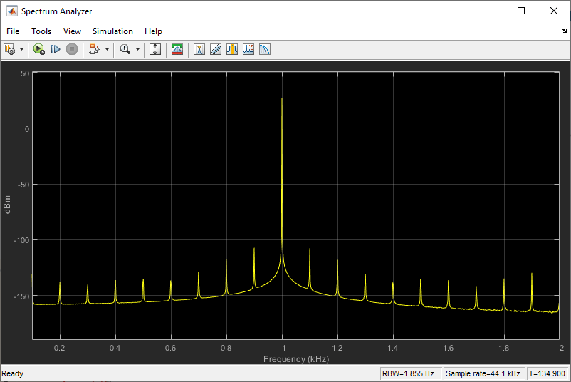
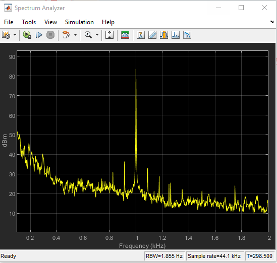
The frequency you set on the Slider is the tallest peak on the Spectrum Analyzer, while the rest of the peaks are the harmonics of this frequency. You can also change the frequency using the Slider and observe the shift in the tallest peak on the Spectrum Analyzer.
Spectrum Analyzer Output
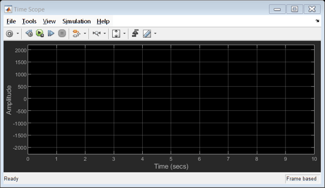
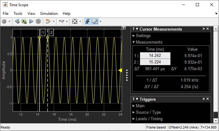
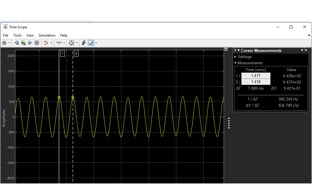
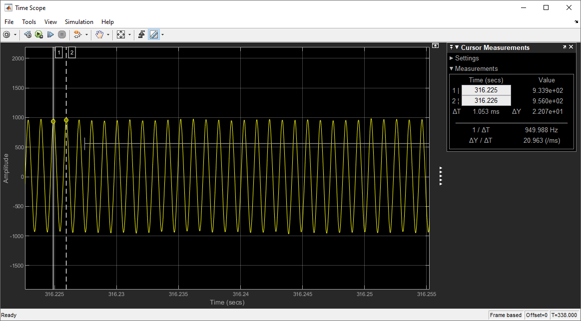
On the Time Scope, you can use the cursors to measure the time delay between two peaks of the audio signal. The inverse of this delay is the frequency of the audio signal.
Time Scope Output
Studying Sampling Frequency and Nyquist Criterion
You can change the sampling frequency of the audio signal and observe the output in the Time Scope to see whether the audio signal is fully reconstructed or not.
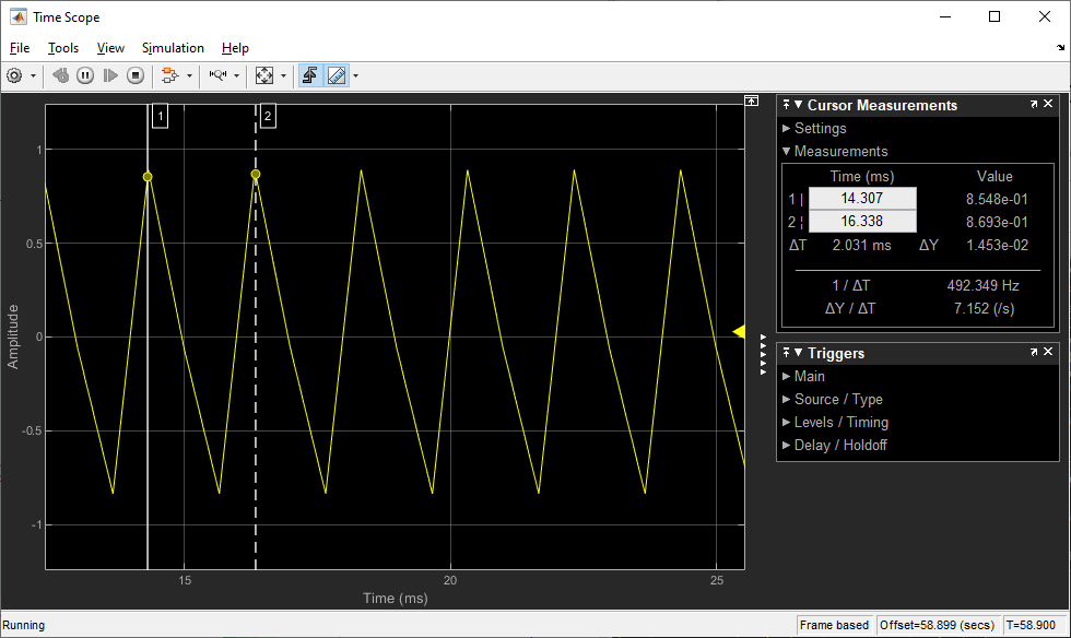
Time scope output view for audio signal set to 1000 Hz and sampling frequency set to 1500 Hz
For the audio signal frequency set to 1000 Hz and the sampling frequency set to 1500 Hz, it does not meet the Nyquist criterion. Follow this procedure to observe this phenomenon.
In the Sine Wave (DSP System Toolbox) block, set Sample time to
1500and Sample per frame to150.In the ALSA Audio Capture block, set Audio sampling frequency to
1500and Samples per frame to150.On the Simulation tab of the Simulink model, click Run.
Open the Time Scope (DSP System Toolbox) block and observe the audio signal. You can see that the reconstructed audio signal does not nearly resemble the original continuous sine wave.
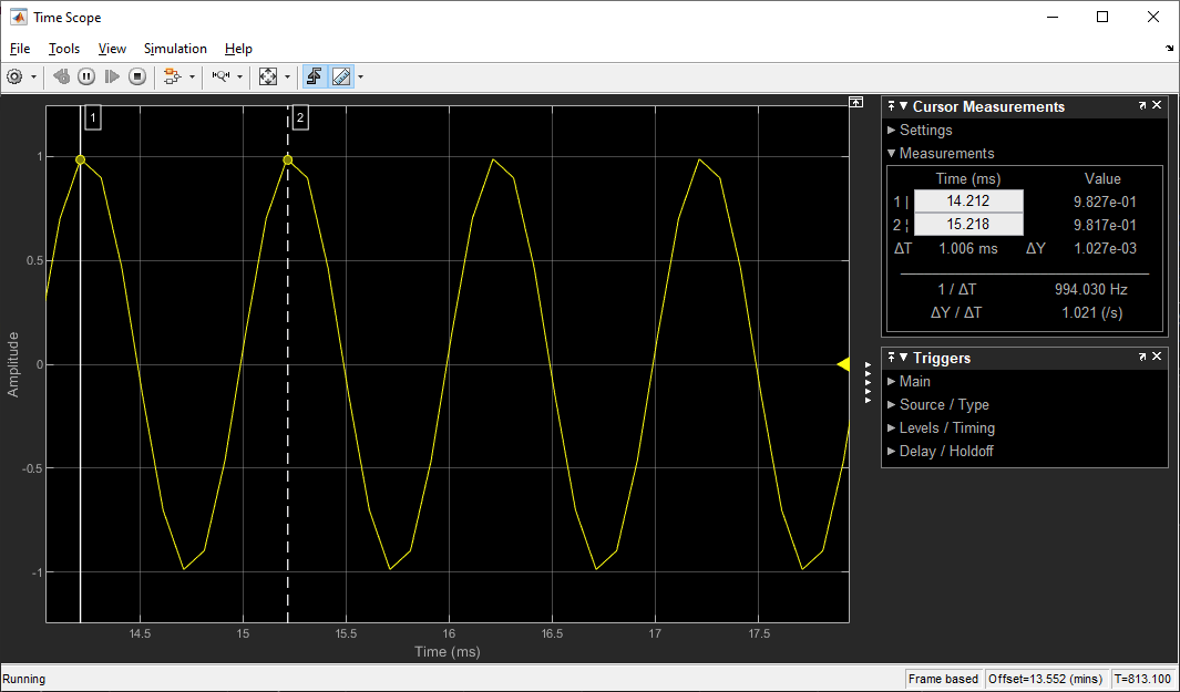
Time scope output view for audio signal set to 1000 Hz and sampling frequency set to 10000 Hz
Set the audio signal frequency to 1000 Hz and the sampling frequency to 10000 Hz so that the audio signal meets the Nyquist criterion.
In the Sine Wave (DSP System Toolbox) block, set Sample time to
10000and Sample per frame to1000.In the ALSA Audio Capture block, set Audio sampling frequency to
10000and Samples per frame to1000.On the Simulation tab of the Simulink model, click Run.
Open the Time Scope (DSP System Toolbox) block and observe the audio signal. You can see that the reconstructed audio signal closely resembles the original continuous sine wave.
Time scope output view for audio signal set to 1000 Hz and sampling frequency set to 44100 Hz
Set the audio signal frequency to 1000 Hz and the sampling frequency to 44100 Hz so that the audio signal meets the Nyquist criterion.
In the Sine Wave (DSP System Toolbox) block, set Sample time to
44100and Sample per frame to4410.In the ALSA Audio Capture block, set Audio sampling frequency to
44100and Samples per frame to4410.On the Simulation tab of the Simulink model, click Run.
Open the Time Scope (DSP System Toolbox) block and observe the audio signal. You can see that the reconstructed audio signal resembles the original continuous sine wave.
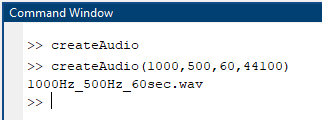
Generate WAV File Using createAudio Function
The createAudio.m file includes the createAudio function that is specific to this example. This function generates a WAV file in the current directory of the example. You can execute the function in the MATLAB Command Window in this format.
createAudio(startFreq, endFreq, duration, samplingFreq)
The createAudio function has three input arguments.
startFreq— Frequency of the audio signal at which it starts.endFreq— Frequency of the audio signal at which it ends.duration— Total duration of the audio signal generated in seconds.samplingFreq— Sampling frequency of the audio signal.
The createAudio|function generates the audio signal with default amplitude set to |1.
Using this function, generate two audio signals with these specifications.
1. Audio signal with the frequency of 1000 Hz, signal duration of 60 seconds, and sampling frequency of 44100 Hz.
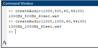
createAudio(1000,1000,60,44100)
This generates a WAV file in the current directory named 1000Hz_1000Hz_60sec.wav.
1. Audio signal that starts at 1000 Hz and ends at 500 Hz, with the signal duration of 60 seconds, and sampling frequency of 44100 Hz.
createAudio(1000,500,60,44100)
This generates a WAV file in the current directory named 1000Hz_500Hz_60sec.wav.
Transfer the 1000Hz_1000Hz_60sec.wav and 1000Hz_500Hz_60sec.wav files to your mobile phone.
Deploy Simulink Model on Raspberry Pi Hardware
1. Position the Manual Switch in the Raspberry Pi Sensors and Inputs area to receive the output from the ALSA Audio Capture block in the Raspberry Pi Sensors and Inputs area.
2. On the Hardware tab of the Simulink model, in the Mode section, select Run on board and then click Monitor & Tune.
3. Play the 1000Hz_1000Hz_60sec.wav file on your mobile phone and place it close to the microphone that is interfaced with the Raspberry Pi hardware board.
3. Observe the output on the Spectrum Analyzer and Time Scope blocks.
Spectrum Analyzer Output
You can observe the noise signals also being captured on the Spectrum Analyzer.
Time Scope Output
5. Play the 1000Hz_500Hz_60sec.wav file on your mobile phone and place it close to the USB microphone that is interfaced with the Raspberry Pi hardware board.
6. Observe the output in the Spectrum Analyzer and Time Scope blocks.
Spectrum Analyzer Output
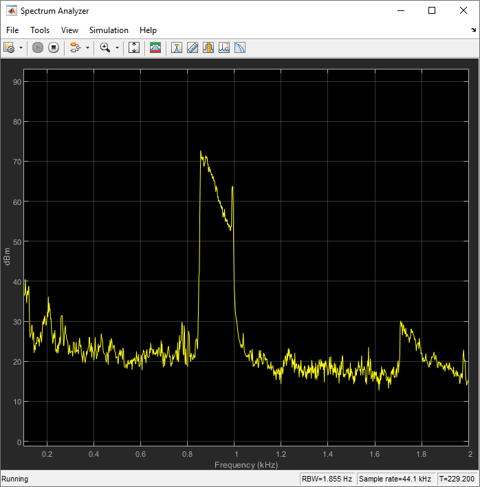
Time Scope Output
Observe the shift in the peak frequency as it drops from 1000 Hz to 500 Hz on the Spectrum Analyzer.
Other Things to Try
Sample the audio signal at a rate lower than Nyquist criterion and observe the aliasing effect in the Spectrum Analyzer.
See Also
You can also select a web site from the following list:
Americas
- América Latina (Español)
- Canada (English)
- United States (English)
Europe
- Belgium (English)
- Denmark (English)
- Deutschland (Deutsch)
- España (Español)
- Finland (English)
- France (Français)
- Ireland (English)
- Italia (Italiano)
- Luxembourg (English)
- Netherlands (English)
- Norway (English)
- Österreich (Deutsch)
- Portugal (English)
- Sweden (English)
- Switzerland
- United Kingdom (English)