predict
Predict labels using discriminant analysis classifier
Description
[ also returns:label,score,cost]
= predict(Mdl,X)
A matrix of classification scores (
score) indicating the likelihood that a label comes from a particular class. For discriminant analysis, scores are posterior probabilities.A matrix of expected classification cost (
cost). For each observation inX, the predicted class label corresponds to the minimum expected classification cost among all classes.
Examples
Predict Class Labels Using Discriminant Analysis Model
Load Fisher's iris data set. Determine the sample size.
load fisheriris
N = size(meas,1);
Partition the data into training and test sets. Hold out 10% of the data for testing.
rng(1); % For reproducibility
cvp = cvpartition(N,'Holdout',0.1);
idxTrn = training(cvp); % Training set indices
idxTest = test(cvp);    % Test set indices
Store the training data in a table.
tblTrn = array2table(meas(idxTrn,:));
tblTrn.Y = species(idxTrn);
Train a discriminant analysis model using the training set and default options.
Mdl = fitcdiscr(tblTrn,'Y');Predict labels for the test set. You trained Mdl using a table of data, but you can predict labels using a matrix.
labels = predict(Mdl,meas(idxTest,:));
Construct a confusion matrix for the test set.
confusionchart(species(idxTest),labels)
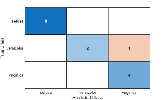
Mdl misclassifies one versicolor iris as virginica in the test set.
Plot Class Posterior Probability Regions
Load Fisher's iris data set. Consider training using the petal lengths and widths only.
load fisheriris
X = meas(:,3:4);
Train a quadratic discriminant analysis model using the entire data set.
Mdl = fitcdiscr(X,species,'DiscrimType','quadratic');
Define a grid of values in the observed predictor space. Predict the posterior probabilities for each instance in the grid.
xMax = max(X);
xMin = min(X);
d = 0.01;
[x1Grid,x2Grid] = meshgrid(xMin(1):d:xMax(1),xMin(2):d:xMax(2));

[~,score] = predict(Mdl,[x1Grid(:),x2Grid(:)]);
Mdl.ClassNames
ans = 3x1 cell
    {'setosa'    }
    {'versicolor'}
    {'virginica' }
score is a matrix of class posterior probabilities. The columns correspond to the classes in Mdl.ClassNames. For example, score(j,1) is the posterior probability that observation j is a setosa iris.
Plot the posterior probability of versicolor classification for each observation in the grid and plot the training data.
figure;
contourf(x1Grid,x2Grid,reshape(score(:,2),size(x1Grid,1),size(x1Grid,2)));
h = colorbar;
clim([0 1]);
colormap jet;
hold on
gscatter(X(:,1),X(:,2),species,'mcy','.x+');
axis tight
title('Posterior Probability of versicolor');
hold off
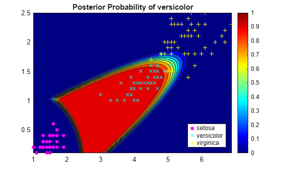
The posterior probability region exposes a portion of the decision boundary.
Input Arguments
Output Arguments
More About
Alternative Functionality
Simulink Block
To integrate the prediction of a discriminant analysis classification model into
Simulink®, you can use the ClassificationDiscriminant
Predict block in the Statistics and Machine Learning Toolbox™ library or a MATLAB® Function block with the predict function. For examples,
see Predict Class Labels Using ClassificationDiscriminant Predict Block and Predict Class Labels Using MATLAB Function Block.
When deciding which approach to use, consider the following:
If you use the Statistics and Machine Learning Toolbox library block, you can use the Fixed-Point Tool (Fixed-Point Designer) to convert a floating-point model to fixed point.
Support for variable-size arrays must be enabled for a MATLAB Function block with the
predictfunction.If you use a MATLAB Function block, you can use MATLAB functions for preprocessing or post-processing before or after predictions in the same MATLAB Function block.
Extended Capabilities
Version History
Introduced in R2011b
See Also
Classes
Functions
You can also select a web site from the following list:
Americas
- América Latina (Español)
- Canada (English)
- United States (English)
Europe
- Belgium (English)
- Denmark (English)
- Deutschland (Deutsch)
- España (Español)
- Finland (English)
- France (Français)
- Ireland (English)
- Italia (Italiano)
- Luxembourg (English)
- Netherlands (English)
- Norway (English)
- Österreich (Deutsch)
- Portugal (English)
- Sweden (English)
- Switzerland
- United Kingdom (English)