신호 미분하기

잡음 전력을 증가시키지 않고 신호를 미분하고자 할 수 있습니다. MATLAB® 함수 diff는 잡음을 증폭시킵니다. 따라서, 그로 인한 부정확성은 미분을 거듭할수록 커집니다. 이 문제를 해결하려면 미분기 필터를 대신 사용하십시오.

지진이 일어나는 동안 건물 바닥의 변위를 분석합니다. 속도와 가속도를 시간 함수로 구합니다.

파일 earthquake를 불러옵니다. 이 파일에는 다음과 같은 변수가 들어 있습니다.

• drift: 바닥 변위(단위: 센티미터)

• t: 시간(단위: 초)

• Fs: 샘플 레이트( = 1kHz)

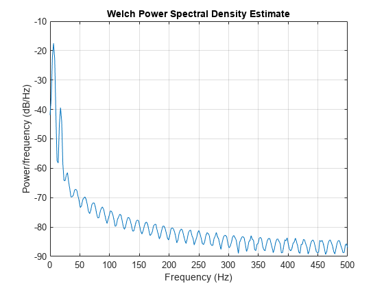
load('earthquake.mat')

pwelch를 사용하여 신호의 파워 스펙트럼 추정값을 표시합니다. 신호 에너지의 대부분이 100Hz 아래의 주파수에 포함되어 있는 것을 확인할 수 있습니다.

pwelch(drift,[],[],[],Fs)

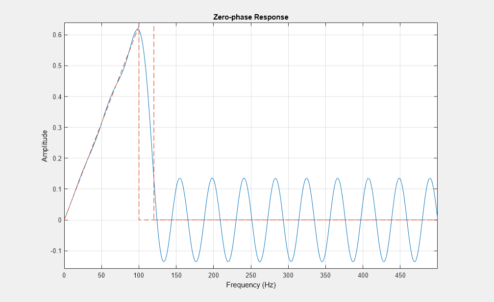
designfilt를 사용하여 차수가 50인 FIR 미분기를 설계합니다. 대부분의 신호 에너지를 포함하기 위해 100Hz의 통과대역 주파수와 120Hz의 저지대역 주파수를 지정합니다. zerophase로 필터를 검사합니다.

Nf = 50; 
Fpass = 100; 
Fstop = 120;

d = designfilt('differentiatorfir','FilterOrder',Nf, ...
    'PassbandFrequency',Fpass,'StopbandFrequency',Fstop, ...
    'SampleRate',Fs);

zerophase(d,[],Fs)

변동을 미분하여 속도를 구합니다. 도함수를 연속 샘플 간 시간 간격(dt)으로 나누어 올바른 단위를 설정합니다.

dt = t(2)-t(1);

vdrift = filter(d,drift)/dt;

필터링된 신호는 지연됩니다. grpdelay를 사용하여 지연이 필터 차수의 절반에 해당하는지 확인합니다. 샘플을 삭제하여 이를 보정합니다.

delay = mean(grpdelay(d))

delay = 25

tt = t(1:end-delay);
vd = vdrift;
vd(1:delay) = [];

출력값에는 길이가 필터 차수와 일치하거나 군지연의 2배에 해당하는 과도(Transient)도 포함됩니다. delay 샘플은 위에서 삭제되었습니다. delay를 더 삭제하여 과도를 제거합니다.

tt(1:delay) = [];
vd(1:delay) = [];

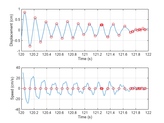
변동과 변동 속도를 플로팅합니다. findpeaks를 사용하여 변동의 최댓값과 최솟값이 도함수의 영점교차에 해당하는지 확인합니다.

[pkp,lcp] = findpeaks(drift);
zcp = zeros(size(lcp));

[pkm,lcm] = findpeaks(-drift);
zcm = zeros(size(lcm));

subplot(2,1,1)
plot(t,drift,t([lcp lcm]),[pkp -pkm],'or')
xlabel('Time (s)')
ylabel('Displacement (cm)')
grid

subplot(2,1,2)
plot(tt,vd,t([lcp lcm]),[zcp zcm],'or')
xlabel('Time (s)')
ylabel('Speed (cm/s)')
grid

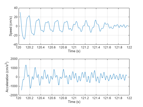
변동 속도를 미분하여 가속도를 구합니다. 지연이 두 배 더 깁니다. 지연을 보정하려면 두 배 많은 샘플을 삭제하고 과도를 제거하려면 동일한 개수의 샘플을 삭제하십시오. 속도와 가속도를 플로팅합니다.

adrift = filter(d,vdrift)/dt;

at = t(1:end-2*delay);
ad = adrift;
ad(1:2*delay) = [];

at(1:2*delay) = [];
ad(1:2*delay) = [];

subplot(2,1,1)
plot(tt,vd)
xlabel('Time (s)')
ylabel('Speed (cm/s)')
grid

subplot(2,1,2)
plot(at,ad)
ax = gca;
ax.YLim = 2000*[-1 1];
xlabel('Time (s)')
ylabel('Acceleration (cm/s^2)')
grid

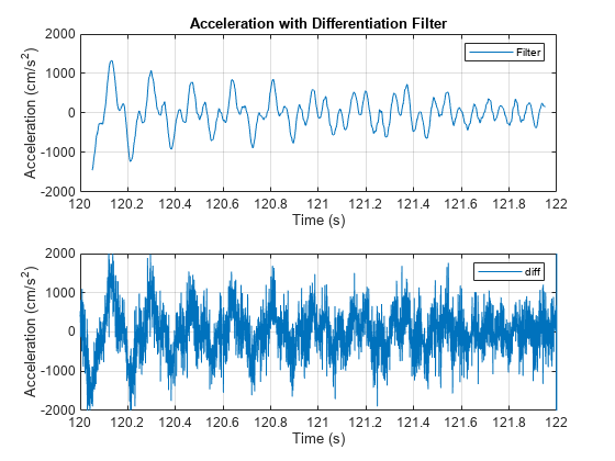
diff를 사용하여 가속도를 계산합니다. 0을 추가하여 배열 크기의 변동을 보정합니다. 이 결과를 필터로 구한 값과 비교합니다. 고주파수 잡음의 크기를 확인합니다.

vdiff = diff([drift;0])/dt;
adiff = diff([vdiff;0])/dt;

subplot(2,1,1)
plot(at,ad)
ax = gca;
ax.YLim = 2000*[-1 1];
xlabel('Time (s)')
ylabel('Acceleration (cm/s^2)')
grid
legend('Filter')
title('Acceleration with Differentiation Filter')

subplot(2,1,2)
plot(t,adiff)
ax = gca;
ax.YLim = 2000*[-1 1];
xlabel('Time (s)')
ylabel('Acceleration (cm/s^2)')
grid
legend('diff')

참고 항목

findpeaks | designfilt | grpdelay | periodogram | zerophase

관련 항목

• 디지털 필터링에 대한 실용적 입문