robstab
Robust stability of uncertain system
Syntax
Description
[ calculates the robust
stability margin for an uncertain system. This stability margin is
relative to the uncertainty level specified in stabmarg,wcu]
= robstab(usys)usys.
A robust stability margin greater than 1 means that the system is
stable for all values of its modeled uncertainty. A robust stability
margin less than 1 means that the system becomes unstable for some
values of the uncertain elements within their specified ranges. For
example, a margin of 0.5 implies the following:
usysremains stable as long as the uncertain element values stay within 0.5 normalized units of their nominal values.There is a destabilizing perturbation of size 0.5 normalized units.
The structure stabmarg contains upper and
lower bounds on the actual stability margin and the critical frequency
at which the stability margin is smallest. The structure wcu contains
the destabilizing values of the uncertain elements.
[ restricts
the robust stability margin computation to the frequencies specified
by stabmarg,wcu]
= robstab(usys,w)w.
If
wis a cell array of the form{wmin,wmax}, thenrobstabrestricts the stability margin computation to the interval betweenwminandwmax.If
wis a vector of frequencies, thenrobstabcomputes the robust stability margin at the specified frequencies only.
[ specifies
additional options for the computation. Use stabmarg,wcu]
= robstab(___,opts)robOptions to
create opts. You can use this syntax with any
of the previous input-argument combinations.
Examples
Robust Stability Margin of Closed-Loop System
Consider a control system whose plant contains both parametric uncertainty and dynamic uncertainty. Create a model of the plant using uncertain elements.
k = ureal('k',10,'Percent',40);
delta = ultidyn('delta',[1 1]);
G = tf(18,[1 1.8 k]) * (1 + 0.5*delta);
Create a model of the controller, and build the closed-loop transfer function.
C = pid(2.3,3,0.38,0.001);
CL = feedback(G*C,1);
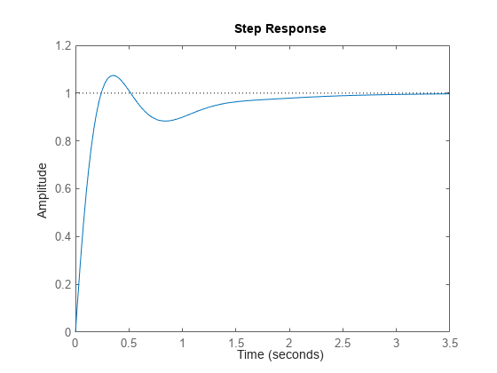
A step response plot shows that the closed-loop system is nominally stable.
step(CL.NominalValue)
Examine the robust stability of the closed-loop system.
[stabmarg,wcu] = robstab(CL);
stabmarg
stabmarg = struct with fields:
           LowerBound: 1.5960
           UpperBound: 1.5993
    CriticalFrequency: 4.8627
The LowerBound and UpperBound fields of stabmarg show the robust stability margin of the closed-loop system is around 1.6. This result means that the system can withstand about 60% more uncertainty than is specified in the uncertain elements without going unstable.
You can use uscale to scale system uncertainty by the stability margin, to examine the system response for the full range of safe uncertainties. Scale the uncertainties in CL by the robust stability margin to create a system with the maximum tolerable amount of uncertainty.
CLmaxunc = uscale(CL,stabmarg.UpperBound);
CLmaxunc.Uncertainty.delta
Uncertain LTI dynamics "delta" with 1 outputs, 1 inputs, and gain less than 1.6.
CLmaxunc.Uncertainty.k
Uncertain real parameter "k" with nominal value 10 and variability [-64,64]%.
The uncertain elements in CLmaxunc have ranges about 1.6 times the range of the original modeled uncertainty in CL.
The output wcu is a structure that contains the smallest perturbation to k and delta that make the system unstable. Confirm the instability by substituting these values into the closed-loop model and examining the pole locations.
CLunst = usubs(CL,wcu);
pole(CLunst)
ans = 8×1 complex
102 ×

  -9.9314 + 0.0000i
  -0.1027 + 0.1009i
  -0.1027 - 0.1009i
  -0.0000 + 0.0486i
  -0.0000 - 0.0486i
  -0.0115 + 0.0000i
  -0.0216 + 0.0000i
  -0.0403 + 0.0000i
The resulting system has an undamped pair of complex poles with natural frequency 4.89, which renders it unstable. The CriticalFrequency field of stabmarg contains the same value, which is the frequency at which the CL is closest to instability.
Sensitivity to Uncertain Elements
Examine the relative sensitivity of the robust stability margin to the uncertain elements of the system. Consider a model of a control system containing uncertain elements.
k = ureal('k',10,'Percent',40);
delta = ultidyn('delta',[1 1]);
G = tf(18,[1 1.8 k]) * (1 + 0.25*delta);
C = pid(2.3,3,0.38,0.001);
CL = feedback(G*C,1);
Create an options set for robstab that enables the sensitivity calculation.
opts = robOptions('Sensitivity','On');
Calculate the robust stability margin, specifying the info output to access additional information about the calculation.
[stabmarg,wcu,info] = robstab(CL,opts);
Examine the Sensitivity field of info.
info.Sensitivity
ans = struct with fields:
    delta: 80
        k: 20
The values in this field indicate how much a change in the normalized perturbation on each element affects the stability margin. For example, the sensitivity for k is 21. This value means that a given change dk in the normalized uncertainty range of k causes a change of about 21% percent of that, or 0.21*dk, in the stability margin. The margin in this case is much more sensitive to delta, for which the margin changes by about 81% of the change in the normalized uncertainty range.
Robust Stability Margin as a Function of Frequency
Consider a model of a control system containing uncertain elements.
k = ureal('k',10,'Percent',40);
delta = ultidyn('delta',[1 1]);
G = tf(18,[1 1.8 k]) * (1 + 0.5*delta);
C = pid(2.3,3,0.38,0.001);
CL = feedback(G*C,1);
By default, robstab computes only the weakest stability margin over all frequencies. To see how the stability margin varies with frequency, use the 'VaryFrequency' option of robOptions. For example, compute the stability margin of the system at frequency points between 0.1 and 10 rad/s.
opts = robOptions('VaryFrequency','on');
[stabmarg,wcu,info] = robstab(CL,{0.1,10},opts);
info
info = struct with fields:
                Model: 1
            Frequency: [19x1 double]
               Bounds: [19x2 double]
    WorstPerturbation: [19x1 struct]
          Sensitivity: [1x1 struct]
robstab returns the vector of frequencies in the info output, in the Frequencies field. info.Bounds contains the upper and lower bounds on the stability margin at each frequency. Use these values to plot the frequency dependence of the stability margin.
semilogx(info.Frequency,info.Bounds)
title('Stability Margin vs. Frequency')
ylabel('Margin')
xlabel('Frequency')
legend('Lower bound','Upper bound')
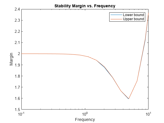
When you use the 'VaryFrequency' option, robstab chooses frequency points automatically. The frequencies it selects are guaranteed to include the frequency at which the stability margin is weakest (within the specified range). Display the returned frequency values to confirm that they include the critical frequency.
info.Frequency
ans = 19×1

    0.1000
    0.1061
    0.1425
    0.1914
    0.2572
    0.3455
    0.4642
    0.6236
    0.8377
    1.1253
      ⋮
stabmarg.CriticalFrequency
ans = 4.8269
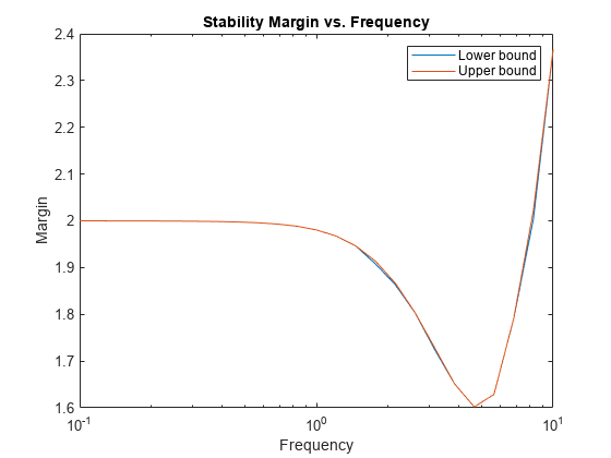
Alternatively, instead of using 'VaryFrequency', you can specify particular frequencies at which to compute the robust stability margins. info.Bounds contains the margins at all specified frequencies. However, these results are not guaranteed to include the weakest margin, which might fall between specified frequency points.
w = logspace(-1,1,25);
[stabmarg,wcu,info] = robstab(CL,w);
semilogx(w,info.Bounds)
title('Stability Margin vs. Frequency')
ylabel('Margin')
xlabel('Frequency')
legend('Lower bound','Upper bound')
Input Arguments
Output Arguments
Algorithms
Computing the robustness margin at a particular frequency is equivalent to computing the structured singular value, μ, for some appropriate block structure (μ-analysis).
For uss and genss models, robstab(usys) and robstab(usys,{wmin,wmax}) use
an algorithm that finds the smallest margin across frequency. This
algorithm does not rely on frequency gridding and is not adversely
affected by discontinuities of the μ structured
singular value. See Getting Reliable Estimates of Robustness Margins for
more information.
For ufrd and genfrd models, robstab computes
the μ lower and upper bounds at each frequency
point. This computation offers no guarantee between frequency points
and can be inaccurate if there are discontinuities or sharp peaks
in μ. The syntax robstab(uss,w),
where w is a vector of frequency points, is the
same as robstab(ufrd(uss,w)) and also relies on
frequency gridding to compute the margin.
In general, the algorithm for state-space models is faster and
safer than the frequency-gridding approach. In some cases, however,
the state-space algorithm requires many μ calculations.
In those cases, specifying a frequency grid as a vector w can
be faster, provided that the robustness margin varies smoothly with
frequency. Such smooth variation is typical for systems with dynamic
uncertainty.
Version History
Introduced in R2016b
You can also select a web site from the following list:
Americas
- América Latina (Español)
- Canada (English)
- United States (English)
Europe
- Belgium (English)
- Denmark (English)
- Deutschland (Deutsch)
- España (Español)
- Finland (English)
- France (Français)
- Ireland (English)
- Italia (Italiano)
- Luxembourg (English)
- Netherlands (English)
- Norway (English)
- Österreich (Deutsch)
- Portugal (English)
- Sweden (English)
- Switzerland
- United Kingdom (English)