robgain
Robust performance of uncertain system
Syntax
Description
[ calculates
the robust performance margin for an uncertain system and the performance
level perfmarg,wcu]
= robgain(usys,gamma)gamma. The performance of usys is
measured by its peak gain or peak singular value (see Robustness and Worst-Case Analysis).
The performance margin is relative to the uncertainty level specified
in usys. A margin greater than 1 means that the
gain of usys remains below gamma for
all values of the uncertainty modeled in usys.
A margin less than 1 means that at some frequency, the gain of usys exceeds gamma for
some values of the uncertain elements within their specified ranges.
For example, a margin of 0.5 implies the following:
The gain of
usysremains belowgammaas long as the uncertain element values stay within 0.5 normalized units of their nominal values.There is a perturbation of size 0.5 normalized units that drives the peak gain to the level
gamma.
The structure perfmarg contains upper and
lower bounds on the actual performance margin and the critical frequency
at which the margin upper bound is smallest. The structure wcu contains
the uncertain-element values that drive the peak gain to the level gamma.
[ assesses
the robust performance margin for the frequencies specified by perfmarg,wcu]
= robgain(usys,gamma,w)w.
If
wis a cell array of the form{wmin,wmax}, thenrobgainrestricts the performance margin computation to the interval betweenwminandwmax.If
wis a vector of frequencies, thenrobgaincomputes the performance margin at the specified frequencies only.
[ specifies
additional options for the computation. Use perfmarg,wcu]
= robgain(___,opts)robOptions to
create opts. You can use this syntax with any
of the previous input-argument combinations.
Examples
Robust Performance of Closed-Loop System
Consider a control system whose plant contains both parametric uncertainty and dynamic uncertainty. Create a model of the plant using uncertain elements.
k = ureal('k',10,'Percent',40);
delta = ultidyn('delta',[1 1]);
G = tf(18,[1 1.8 k]) * (1 + 0.5*delta);
Create a model of the controller, and build the closed-loop sensitivity function, S. The sensitivity measures the closed-loop response at the plant output to a disturbance at the plant input.
C = pid(2.3,3,0.38,0.001);
S = feedback(1,G*C);
bodemag(S,S.NominalValue)
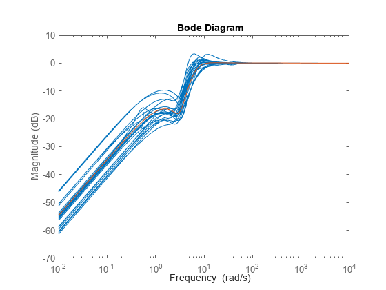
The peak gain of the nominal response is very nearly 1, but some of the sampled systems within the uncertainty range exceed that level. Suppose that you can tolerate some ringdown in the response but do not want the peak gain to exceed 1.5. Use robgain to find out how much uncertainty the system can have while the peak gain remains below 1.5.
[perfmarg,wcu] = robgain(S,1.5);
perfmarg
perfmarg = struct with fields:
           LowerBound: 0.7821
           UpperBound: 0.7837
    CriticalFrequency: 7.8566
The LowerBound and UpperBound fields of perfmarg show that the robust performance margin is around 0.78. This result means that there is a perturbation of only about 78% of the uncertainty specified in S with peak gain exceeding 1.5.
You can use uscale to examine what that normalized uncertainty of 78% means in terms of actual ranges of uncertainty. Scale all the uncertain elements in S to create a model of the closed-loop system with the maximum level of uncertainty that meets the performance requirement.
factor = perfmarg.LowerBound;
S_scaled = uscale(S,factor)
Uncertain continuous-time state-space model with 1 outputs, 1 inputs, 4 states.
The model uncertainty consists of the following blocks:
  delta: Uncertain 1x1 LTI, peak gain = 0.782, 1 occurrences
  k: Uncertain real, nominal = 10, variability = [-31.3,31.3]%, 1 occurrences

Type "S_scaled.NominalValue" to see the nominal value and "S_scaled.Uncertainty" to interact with the uncertain elements.
The display shows how the uncertain elements in S_scaled have changed: the peak gain of the ultidyn element delta is reduced from 1 to 0.78, and the range of variation of the uncertain real parameter k is reduced from ±40% to ±31.3%.
The output wcu is a structure that contains the perturbations to k and delta that correspond to the target maximum performance of 1.5. Verify that the values in wcu cause Smax to achieve the gain level of 1.5 by substituting them into S.
Smax = usubs(S,wcu);
getPeakGain(Smax,1e-6)
ans = 1.5001
Examine the disturbance rejection of the system with these values.
step(S.NominalValue,Smax)
legend('Nominal','Peak Gain = 1.5')
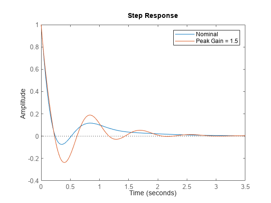
The CriticalFrequency field of perfmarg contains the frequency at which the peak gain reaches 1.5.
Sensitivity of Performance to Uncertain Elements
Examine the relative sensitivity of the robust performance margin to the uncertain elements of the system. Consider a model of a control system containing uncertain elements.
k = ureal('k',10,'Percent',50);
delta = ultidyn('delta',[1 1]);
G = tf(18,[1 1.8 k]) * (1 + 0.15*delta);
C = pid(2.3,3,0.38,0.001);
S = feedback(1,G*C);
Create an options set for robgain that enables the sensitivity calculation.
opts = robOptions('Sensitivity','On');
Calculate the robust performance margin of the system relative to a peak gain of 1.5, specifying the info output to access additional information about the calculation.
[perfmarg,wcu,info] = robgain(S,1.5,opts);
Examine the Sensitivity field of info.
info.Sensitivity
ans = struct with fields:
    delta: 75
        k: 28
The values in this field indicate how much a change in the normalized perturbation on each element affects the performance margin. For example, the sensitivity for k is 28. This value means that a given change dk in the normalized uncertainty range of k causes a change of about 28% of that, or 0.28*dk, in the performance margin. The margin in this case is more sensitive to delta, for which the margin changes by about 75% of the change in the normalized uncertainty range.
Robust Performance Margin as a Function of Frequency
Consider a model of a control system containing uncertain elements.
k = ureal('k',10,'Percent',40);
delta = ultidyn('delta',[1 1]);
G = tf(18,[1 1.8 k]) * (1 + 0.5*delta);
C = pid(2.3,3,0.38,0.001);
S = feedback(1,G*C);
By default, robgain computes only the weakest performance margin over all frequencies. To see how the margin varies with frequency, use the 'VaryFrequency' option of robOptions. For example, compute the performance margin of the system for a performance level of 1.5, at frequency points between 0.1 and 100 rad/s.
opts = robOptions('VaryFrequency','on');
[perfmarg,wcu,info] = robgain(S,1.5,{0.1,100},opts);
info
info = struct with fields:
                Model: 1
            Frequency: [32x1 double]
               Bounds: [32x2 double]
    WorstPerturbation: [32x1 struct]
          Sensitivity: [1x1 struct]
robgain returns the vector of frequencies in the info output, in the Frequencies field. info.Bounds contains the upper and lower bounds on the performance margin at each frequency. Use these values to plot the frequency dependence of the performance margin.
semilogx(info.Frequency,info.Bounds)
title('Performance Margin vs. Frequency')
ylabel('Margin')
xlabel('Frequency')
legend('Lower bound','Upper bound')
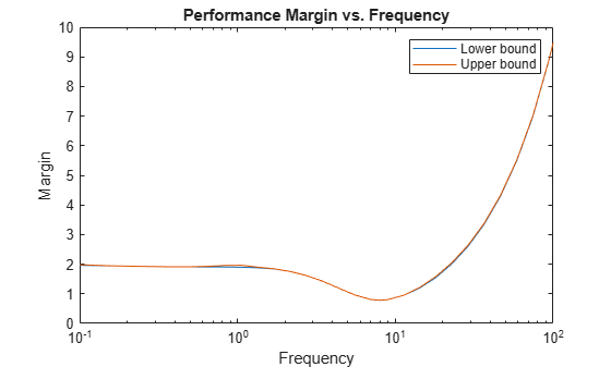
When you use the 'VaryFrequency' option, robgain chooses frequency points automatically. The frequencies it selects are guaranteed to include the frequency at which the margin is smallest (within the specified range). Display the returned frequency values to confirm that they include the critical frequency.
info.Frequency
ans = 32×1

    0.1000
    0.1266
    0.1604
    0.2031
    0.2572
    0.3257
    0.4125
    0.5223
    0.6615
    0.8377
      ⋮
perfmarg.CriticalFrequency
ans = 7.9966
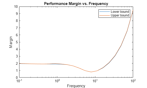
Alternatively, instead of using 'VaryFrequency', you can specify particular frequencies at which to compute the robust performance margins. info.Bounds contains the margins at all specified frequencies. However, these results are not guaranteed to include the weakest margin, which might fall between specified frequency points.
w = logspace(-1,2,20);
[perfmarg,wcu,info] = robgain(S,1.5,w);
semilogx(w,info.Bounds)
title('Performance Margin vs. Frequency')
ylabel('Margin')
xlabel('Frequency')
legend('Lower bound','Upper bound')
Input Arguments
Output Arguments
Algorithms
Computing the robustness margin at a particular frequency is equivalent to computing the structured singular value, μ, for some appropriate block structure (μ-analysis).
For uss and genss models, robgain(usys) and robgain(usys,{wmin,wmax}) use
an algorithm that finds the smallest margin across frequency. This
algorithm does not rely on frequency gridding and is not adversely
affected by discontinuities of the μ structured
singular value. See Getting Reliable Estimates of Robustness Margins for
more information.
For ufrd and genfrd models, robgain computes
the μ lower and upper bounds at each frequency
point. This computation offers no guarantee between frequency points
and can be inaccurate if there are discontinuities or sharp peaks
in μ. The syntax robgain(uss,w),
where w is a vector of frequency points, is the
same as robgain(ufrd(uss,w)) and also relies on
frequency gridding to compute the margin.
In general, the algorithm for state-space models is faster and
safer than the frequency-gridding approach. In some cases, however,
the state-space algorithm requires many μ calculations.
In those cases, specifying a frequency grid as a vector w can
be faster, provided that the robustness margin varies smoothly with
frequency. Such smooth variation is typical for systems with dynamic
uncertainty.
Version History
Introduced in R2016b
You can also select a web site from the following list:
Americas
- América Latina (Español)
- Canada (English)
- United States (English)
Europe
- Belgium (English)
- Denmark (English)
- Deutschland (Deutsch)
- España (Español)
- Finland (English)
- France (Français)
- Ireland (English)
- Italia (Italiano)
- Luxembourg (English)
- Netherlands (English)
- Norway (English)
- Österreich (Deutsch)
- Portugal (English)
- Sweden (English)
- Switzerland
- United Kingdom (English)