step

Display time-varying magnitude response

Since R2018b

Syntax

step(dfv,filt)

step(dfv,B,A)

Description

step(dfv,filt) displays the time-varying magnitude response of the object filter, filt, in the Dynamic Filter Visualizer figure, as long as filt has a valid freqz() implementation.

step(dfv,B,A) displays the magnitude response for the digital filters with numerator and denominator polynomial coefficients stored in B1 and A1, B2 and A2, ..., and BN and AN, respectively.

Examples

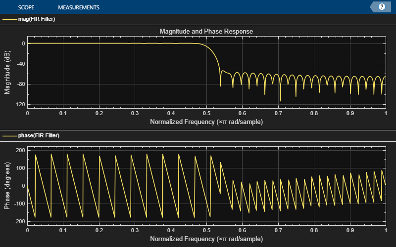
Plot Time-Varying Magnitude and Phase Response of FIR Filter

Design an FIR filter with a time-varying magnitude and phase response. Plot this varying response on a dynamic filter visualizer in normalized frequency units.

Create a dsp.DynamicFilterVisualizer object. Set the PlotAsMagnitudePhase and the NormalizedFrequency properties to true.

dfv = dsp.DynamicFilterVisualizer(PlotAsMagnitudePhase=1,...
    NormalizedFrequency=true,ShowLegend=true,...
    Title='Magnitude and Phase Response',...
    FilterNames="FIR Filter")

dfv = 
  dsp.DynamicFilterVisualizer with properties:

               FFTLength: 2048
     NormalizedFrequency: 1
          FrequencyRange: [0 1]
                  XScale: 'Linear'
        MagnitudeDisplay: 'Magnitude (dB)'
    PlotAsMagnitudePhase: 1
                PlotType: 'Line'
             AxesScaling: 'Auto'

  Show all properties

Vary the cutoff frequency of the FIR filter k from 0.1 to 0.5 in increments of 0.001. View the varying magnitude and phase response using the dynamic filter visualizer.

for k = 0.1:0.001:0.5
    b = fir1(90,k);
    dfv(b,1);
end

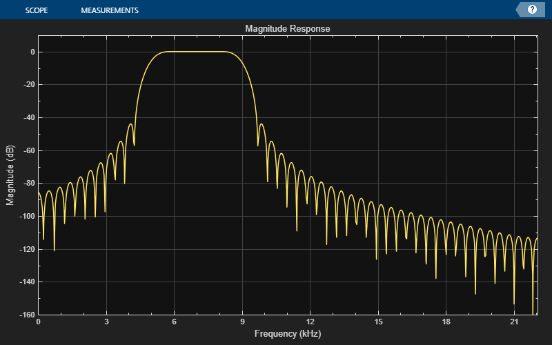
Plot Time-Varying Magnitude Response of Variable Bandwidth FIR Filter

Visualize the varying magnitude response of the variable bandwidth FIR filter using the dynamic filter visualizer.

Create a dsp.DynamicFilterVisualizer object.

dfv = dsp.DynamicFilterVisualizer(YLimits=[-160 10],...
    FilterNames="Variable Bandwidth FIR Filter")

dfv = 
  dsp.DynamicFilterVisualizer with properties:

               FFTLength: 2048
     NormalizedFrequency: 0
              SampleRate: 44100
          FrequencyRange: [0 22050]
                  XScale: 'Linear'
        MagnitudeDisplay: 'Magnitude (dB)'
    PlotAsMagnitudePhase: 0
                PlotType: 'Line'
             AxesScaling: 'Manual'

  Show all properties

Design a bandpass variable bandwidth FIR filter with a center frequency of 5 kHz and a bandwidth of 4 kHz.

Fs = 44100;
vbw = dsp.VariableBandwidthFIRFilter(FilterType='Bandpass',...
    FilterOrder=100,...
    SampleRate=Fs,...
    CenterFrequency=5e3,...
    Bandwidth=4e3);

Vary the center frequency of the filter. Visualize the varying magnitude response of the filter using the dsp.DynamicFilterVisualizer object.

for idx  = 1:100
    dfv(vbw);
    vbw.CenterFrequency = vbw.CenterFrequency + 20;
end

Input Arguments

dfv — Dynamic filter visualizer

dsp.DynamicFilterVisualizer object

Dynamic filter visualizer, specified as a dsp.DynamicFilterVisualizer object.

filt — Filter

filter System object™

Filter System object with a valid freqz() implementation.

B — Numerator polynomial coefficients

row vector

Numerator polynomial coefficients, specified as a row vector.

Data Types: single | double

A — Denominator polynomial coefficients

scalar | row vector

Denominator polynomial coefficients, specified as a:

• scalar –– The filter is an FIR filter.

• row vector –– The filter is an IIR filter.

Data Types: single | double

Version History

Introduced in R2018b