Design Yaw Damper for Jet Transport
Overview of This Case Study
This case study demonstrates the tools for classical control design by stepping through the design of a yaw damper for a 747® jet transport aircraft.
Creating the Jet Model
The jet model during cruise flight at MACH = 0.8 and H = 40,000 ft. is
A=[-.0558 -.9968 .0802 .0415;
     .598 -.115 -.0318 0;
    -3.05 .388 -.4650 0;
        0 0.0805 1 0];

B=[ .00729  0;
   -0.475   0.00775;
    0.153   0.143;
     0      0];

C=[0 1 0 0;
   0 0 0 1];

D=[0 0;
   0 0];

sys = ss(A,B,C,D);
The following commands specify this state-space model as an LTI object and attach names to the states, inputs, and outputs.
states = {'beta' 'yaw' 'roll' 'phi'};
inputs = {'rudder' 'aileron'};
outputs = {'yaw' 'bank angle'};

sys = ss(A,B,C,D,'statename',states,...
                 'inputname',inputs,...
                 'outputname',outputs);
You can display the LTI model sys by typing
sys. This command produces the following result.
a =
            beta      yaw     roll      phi
   beta  -0.0558  -0.9968   0.0802   0.0415
   yaw     0.598   -0.115  -0.0318        0
   roll    -3.05    0.388   -0.465        0
   phi         0   0.0805        1        0

b =
          rudder  aileron
   beta  0.00729        0
   yaw    -0.475  0.00775
   roll    0.153    0.143
   phi         0        0

c =
               beta   yaw  roll   phi
   yaw            0     1     0     0
   bank angle     0     0     0     1

d =
                rudder  aileron
   yaw               0        0
   bank angle        0        0

Continuous-time model.
The model has two inputs and two outputs. The units are radians for
beta (sideslip angle) and phi (bank angle)
and radians/sec for yaw (yaw rate) and roll
(roll rate). The rudder and aileron deflections are in radians as well.
Computing Open-Loop Poles
Compute the open-loop poles and plot them in the s-plane.
>> damp(sys)

         Pole              Damping       Frequency      Time Constant
                                       (rad/seconds)      (seconds)

 -7.28e-03                 1.00e+00       7.28e-03         1.37e+02
 -5.63e-01                 1.00e+00       5.63e-01         1.78e+00
 -3.29e-02 + 9.47e-01i     3.48e-02       9.47e-01         3.04e+01
 -3.29e-02 - 9.47e-01i     3.48e-02       9.47e-01         3.04e+01

pzmap(sys)
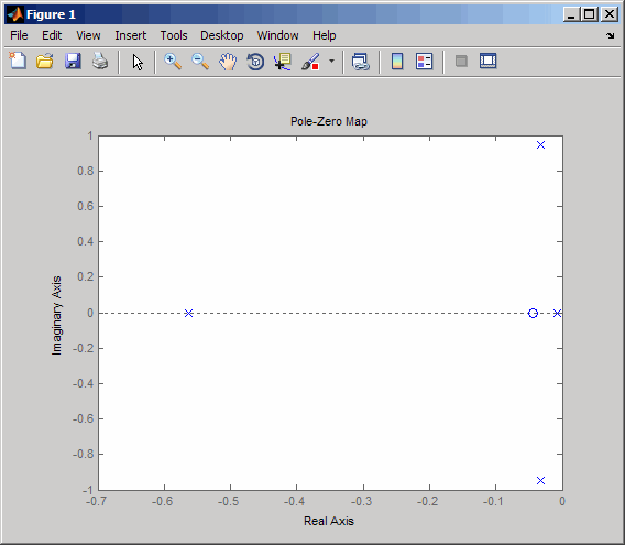
This model has one pair of lightly damped poles. They correspond to what is called the "Dutch roll mode."
Suppose you want to design a compensator that increases the damping of these poles, so that the resulting complex poles have a damping ratio ζ > 0.35 with natural frequency ωn < 1 rad/sec. You can do this using the Control System Toolbox™ analysis tools.
Open-Loop Analysis
First, perform some open-loop analysis to determine possible control strategies.
Start with the time response (you could use step or
impulse here).
impulse(sys)
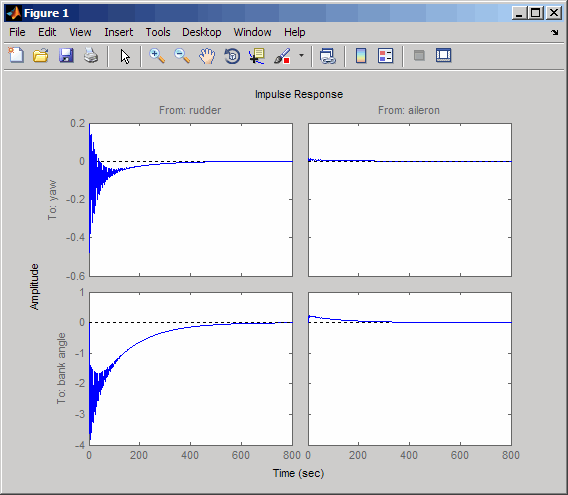
The impulse response confirms that the system is lightly damped. But the time frame is much too long because the passengers and the pilot are more concerned about the behavior during the first few seconds rather than the first few minutes. Next look at the response over a smaller time frame of 20 seconds.
impulse(sys,20)
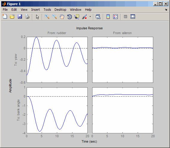
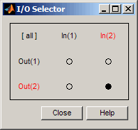
Look at the plot from aileron (input 2) to bank angle (output 2). To show only this plot, right-click and choose I/O Selector, then click on the (2,2) entry. The I/O Selector should look like this.
The new figure is shown below.
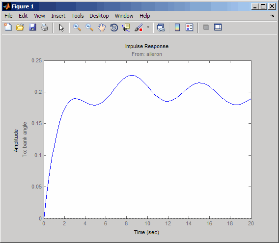
The aircraft is oscillating around a nonzero bank angle. Thus, the aircraft is turning in response to an aileron impulse. This behavior will prove important later in this case study.
Typically, yaw dampers are designed using the yaw rate as sensed output and the rudder as control input. Look at the corresponding frequency response.
sys11=sys('yaw','rudder') % Select I/O pair.
bode(sys11)
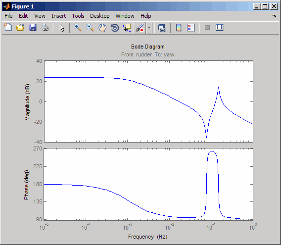
From this Bode diagram, you can see that the rudder has significant effect around the lightly damped Dutch roll mode (that is, near ω = 1 rad/sec).
Root Locus Design
A reasonable design objective is to provide a damping ration ζ > 0.35 with a natural frequency ωn < 1.0 rad/sec. Since the simplest compensator is a static gain, first try to determine appropriate gain values using the root locus technique.
% Plot the root locus for the rudder to yaw channel
rlocus(sys11)
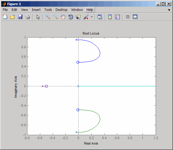
This is the root locus for negative feedback and shows that the system goes unstable almost immediately. If, instead, you use positive feedback, you may be able to keep the system stable.
rlocus(-sys11)
sgrid
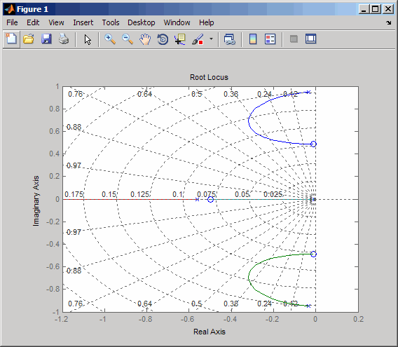
This looks better. By using simple feedback, you can achieve a damping ratio of ζ > 0.45. Click on the blue curve and move the data marker to track the gain and damping values. To achieve a 0.45 damping ratio, the gain should be about 2.85. This figure shows the data marker with similar values.

Next, close the SISO feedback loop.
K = 2.85;
cl11 = feedback(sys11,-K);  % Note: feedback assumes negative
                            % feedback by default
Plot the closed-loop impulse response for a duration of 20 seconds, and compare it to the open-loop impulse response.
impulse(sys11,'b--',cl11,'r',20)

The closed-loop response settles quickly and does not oscillate much, particularly when compared to the open-loop response.
Now close the loop on the full MIMO model and see how the response from the
aileron looks. The feedback loop involves input 1 and output 1 of the plant (use
feedback with index vectors selecting this input/output
pair). At the MATLAB® prompt, type
cloop = feedback(sys,-K,1,1);
damp(cloop)   % closed-loop poles

         Pole              Damping       Frequency      Time Constant
                                       (rad/seconds)      (seconds)

 -3.42e-01                 1.00e+00       3.42e-01         2.92e+00
 -2.97e-01 + 6.06e-01i     4.40e-01       6.75e-01         3.36e+00
 -2.97e-01 - 6.06e-01i     4.40e-01       6.75e-01         3.36e+00
 -1.05e+00                 1.00e+00       1.05e+00         9.50e-01
Plot the MIMO impulse response.
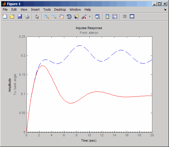
impulse(sys,'b--',cloop,'r',20)
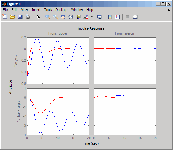
The yaw rate response is now well damped, but look at the plot from aileron (input 2) to bank angle (output 2). When you move the aileron, the system no longer continues to bank like a normal aircraft. You have over-stabilized the spiral mode. The spiral mode is typically a very slow mode and allows the aircraft to bank and turn without constant aileron input. Pilots are used to this behavior and will not like your design if it does not allow them to fly normally. This design has moved the spiral mode so that it has a faster frequency.
Washout Filter Design
What you need to do is make sure the spiral mode does not move further into the left-half plane when you close the loop. One way flight control designers have addressed this problem is to use a washout filter kH(s) where
The washout filter places a zero at the origin, which constrains the spiral mode
pole to remain near the origin. We choose α = 0.2 for a time constant of five
seconds and use the root locus technique to select the filter gain
H. First specify the fixed part
s/(s + α) of the washout by
H = zpk(0,-0.2,1);
Connect the washout in series with the design model sys11 (relation between
input 1 and output 1) to obtain the open-loop model
oloop = H * sys11;
and draw another root locus for this open-loop model.
rlocus(-oloop)
sgrid
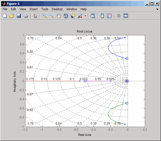
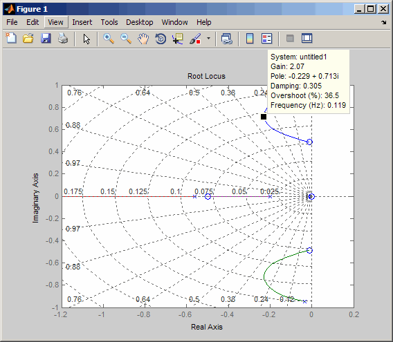
Create and drag a data marker around the upper curve to locate the maximum damping, which is about ζ = 0.3.
This figure shows a data marker at the maximum damping ratio; the gain is approximately 2.07.
Look at the closed-loop response from rudder to yaw rate.
K = 2.07;
cl11 = feedback(oloop,-K);
impulse(cl11,20)

The response settles nicely but has less damping than your previous design. Finally, you can verify that the washout filter has fixed the spiral mode problem. First form the complete washout filter kH(s) (washout + gain).
WOF = -K * H;
Then close the loop around the first I/O pair of the MIMO model
sys and simulate the impulse response.
cloop = feedback(sys,WOF,1,1);

% Final closed-loop impulse response
impulse(sys,'b--',cloop,'r',20)
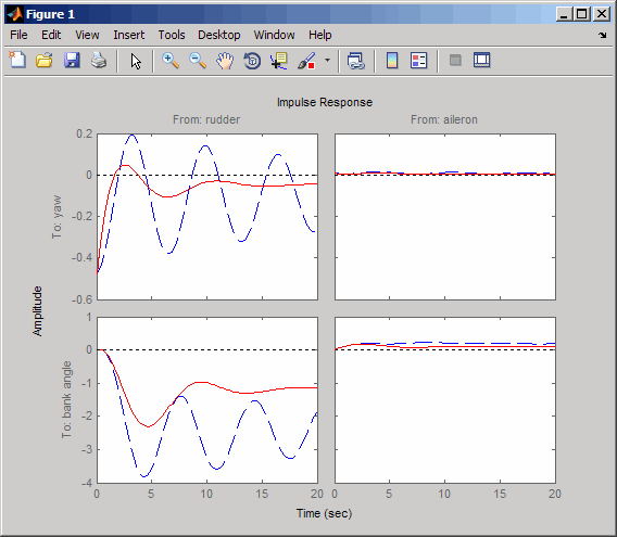
The bank angle response (output 2) due to an aileron impulse (input 2) now has the desired nearly constant behavior over this short time frame. To inspect the response more closely, use the I/O Selector in the right-click menu to select the (2,2) I/O pair.
Although you did not quite meet the damping specification, your design has increased the damping of the system substantially and now allows the pilot to fly the aircraft normally.
