impulse
Impulse response plot of dynamic system; impulse response data
Syntax
Description
[
computes the response from y,tOut] = impulse(sys,[t0,tFinal])t0 to tFinal. For
response configurations config with an impulse delay
td, the function applies the impulse at time t =
t0 + td. (since R2023b)
[
specifies additional options for computing the impulse response, such as the amplitude or
input offset. Use y,tOut] = impulse(___,config)RespConfig to create the option set config. You
can use config with any of the previous input-argument and
output-argument combinations.
impulse( plots the
impulse response of sys,___)sys. This syntax is equivalent to
impulseplot(sys,__). When you need additional plot customization
options, use impulseplot instead.
Examples
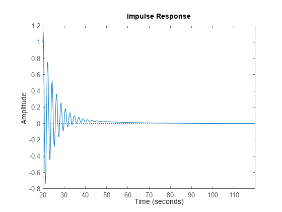
Impulse Response of Dynamic System
Plot the impulse response of a continuous-time system represented by the following transfer function.
For this example, create a tf model that represents the transfer function. You can similarly plot the impulse response of other dynamic system model types, such as zero-pole gain (zpk) or state-space (ss) models.
sys = tf(4,[1 2 10]);
Plot the impulse response.
impulse(sys)
The impulse plot automatically includes a dotted horizontal line indicating the steady-state response. In a MATLAB® figure window, you can right-click on the plot to view other impulse-response characteristics such as peak response and transient time.
Impulse Response of Discrete-Time System
Plot the impulse response of a discrete-time system. The system has a sample time of 0.2 s and is represented by the following state-space matrices.
A = [1.6 -0.7;
      1  0];
B = [0.5; 0];
C = [0.1 0.1];
D = 0;
Create the state-space model and plot its impulse response.
sys = ss(A,B,C,D,0.2);
impulse(sys)
The impulse response reflects the discretization of the model, as it shows the response as computed every 0.2 seconds.
Impulse Response at Specified Times
Examine the impulse response of the following zero-pole-gain model.
sys = zpk(-1,[-0.2+3j,-0.2-3j],1) * tf([1 1],[1 0.05])
sys =

            (s+1)^2
  ----------------------------
  (s+0.05) (s^2 + 0.4s + 9.04)

Continuous-time zero/pole/gain model.
impulse(sys)
By default, impulse chooses an end time that shows the steady state that the response is trending toward. To get a closer look at the transient response, limit the impulse plot to t = 20 s.
impulse(sys,20)
Alternatively, you can specify the exact times at which you want to examine the impulse response, provided they are separated by a constant interval. For instance, examine the response from the end of the transient until the system reaches steady state.
t = 20:0.2:120;
impulse(sys,t)
Even though this plot begins at t = 20, impulse always applies the impulse input at t = 0.
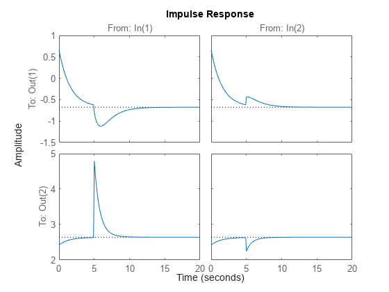
Impulse Response Plot of MIMO Systems
Consider the following second-order state-space model:
A = [-0.5572,-0.7814;0.7814,0];
B = [1,-1;0,2];
C = [1.9691,6.4493];
sys = ss(A,B,C,0);
This model has two inputs and one output, so it has two channels: from the first input to the output and from the second input to the output. Each channel has its own impulse response.
When you use impulse, it computes the responses of all channels.
impulse(sys)
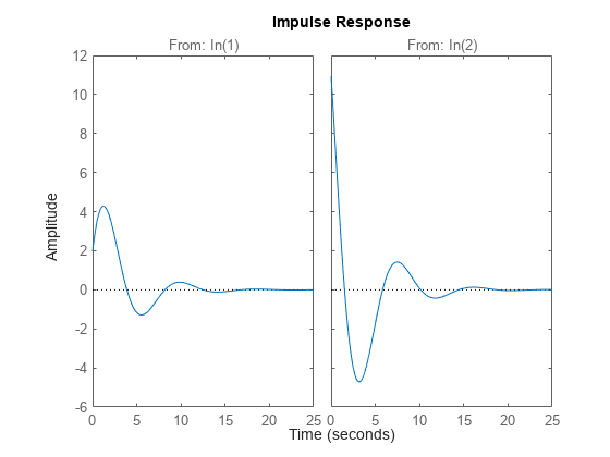
The left plot shows the impulse response of the first input channel, and the right plot shows the impulse response of the second input channel. Whenever you use impulse to plot the responses of a MIMO model, it generates an array of plots representing all the I/O channels of the model. For instance, create a random state-space model with five states, three inputs, and two outputs, and plot its impulse response.
sys = rss(5,2,3);
impulse(sys)
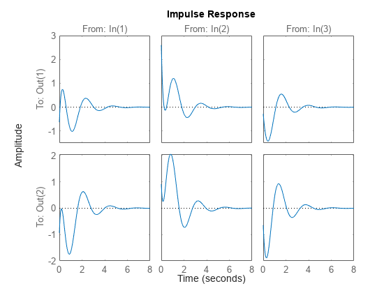
In a MATLAB figure window, you can restrict the plot to a subset of channels by right-clicking on the plot and selecting I/O Selector.
Compare Impulse Response of Multiple Systems
impulse allows you to plot the responses of multiple dynamic systems on the same axis. For instance, compare the closed-loop response of a system with a PI controller and a PID controller. Create a transfer function of the system and tune the controllers.
H = tf(4,[1 2 10]);
C1 = pidtune(H,'PI');
C2 = pidtune(H,'PID');
Form the closed-loop systems and plot their impulse responses.
sys1 = feedback(H*C1,1);
sys2 = feedback(H*C2,1);
impulse(sys1,sys2)
legend('PI','PID','Location','SouthEast')
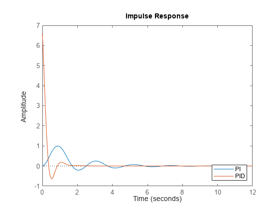
By default, impulse chooses distinct colors for each system that you plot. You can specify colors and line styles using the LineSpec input argument.
 impulse(sys1,'r--',sys2,'b')
 legend('PI','PID','Location','SouthEast')
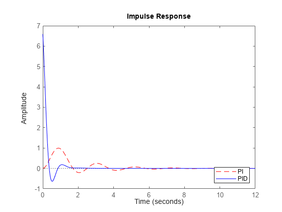
The first LineSpec 'r--' specifies a dashed red line for the response with the PI controller. The second LineSpec 'b' specifies a solid blue line for the response with the PID controller. The legend reflects the specified colors and linestyles. For more plot customization options, use impulseplot.
Impulse Response of Systems in a Model Array
The example Compare Impulse Response of Multiple Systems shows how to plot responses of several individual systems on a single axis. When you have multiple dynamic systems arranged in a model array, impulse plots all their responses at once.
Create a model array. For this example, use a one-dimensional array of second-order transfer functions having different natural frequencies. First, preallocate memory for the model array. The following command creates a 1-by-5 row of zero-gain SISO transfer functions. The first two dimensions represent the model outputs and inputs. The remaining dimensions are the array dimensions.
sys = tf(zeros(1,1,1,5));
Populate the array.
w0 = 1.5:1:5.5;    % natural frequencies
zeta = 0.5;        % damping constant
for i = 1:length(w0)
   sys(:,:,1,i) = tf(w0(i)^2,[1 2*zeta*w0(i) w0(i)^2]);
end
(For more information about model arrays and how to create them, see Model Arrays.) Plot the impulse responses of all models in the array.
impulse(sys)
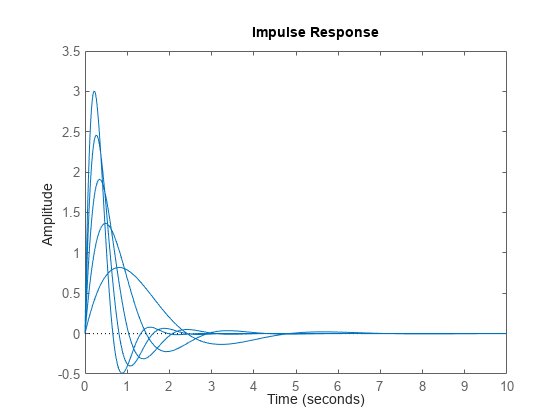
impulse uses the same linestyle for the responses of all entries in the array. One way to distinguish among entries is to use the SamplingGrid property of dynamic system models to associate each entry in the array with the corresponding w0 value.
sys.SamplingGrid = struct('frequency',w0);Now, when you plot the responses in a MATLAB figure window, you can click a trace to see which frequency value it corresponds to.
Impulse Response Data
When you give it an output argument, impulse returns an array of response data. For a SISO system, the response data is returned as a column vector of length equal to the number of time points at which the response is sampled. You can provide the vector t of time points, or allow impulse to select time points for you based on system dynamics. For instance, extract the impulse response of a SISO system at 101 time points between t = 0 and t = 5 s.
sys = tf(4,[1 2 10]);
t = 0:0.05:5;
y = impulse(sys,t);
size(y)
ans = 1×2

   101     1
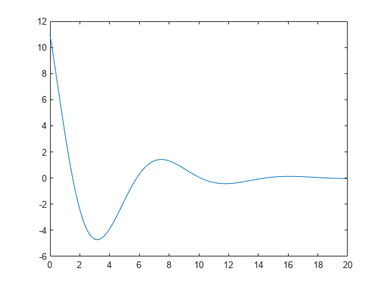
For a MIMO system, the response data is returned in an array of dimensions N-by-Ny-by-Nu, where Ny and Nu are the number of outputs and inputs of the dynamic system. For instance, consider the following state-space model, representing a two-input, one-output system.
A = [-0.5572,-0.7814;0.7814,0];
B = [1,-1;0,2];
C = [1.9691,6.4493];
sys = ss(A,B,C,0);
Extract the impulse response of this system at 200 time points between t = 0 and t = 20 s.
t = linspace(0,20,200);
y = impulse(sys,t);
size(y)
ans = 1×3

   200     1     2
y(:,i,j) is a column vector containing the impulse response from the jth input to the ith output at the times t. For instance, extract the impulse response from the second input to the output.
y12 = y(:,1,2);
plot(t,y12)
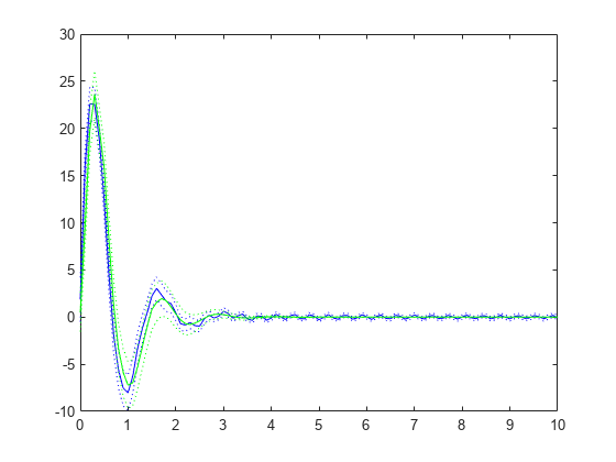
Impulse Responses of Identified Models with Confidence Regions
Compare the impulse response of a parametric identified model to a non-parametric (empirical) model. Also view their 3 confidence regions.
Load the data.
load iddata1 z1
Estimate a parametric model.
sys1 = ssest(z1,4);
Estimate a non-parametric model.
sys2 = impulseest(z1);
Plot the impulse responses for comparison.
t = (0:0.1:10)';
[y1, ~, ~, ysd1] = impulse(sys1,t);
[y2, ~, ~, ysd2] = impulse(sys2,t);
plot(t, y1, 'b', t, y1+3*ysd1, 'b:', t, y1-3*ysd1, 'b:')
hold on
plot(t, y2, 'g', t, y2+3*ysd2, 'g:', t, y2-3*ysd2, 'g:')
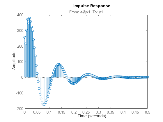
Impulse Response of Identified Time-Series Model
Compute the impulse response of an identified time-series model.
A time-series model, also called a signal model, is one without measured input signals. The impulse plot of this model uses its (unmeasured) noise channel as the input channel to which the impulse signal is applied.
Load the data.
load iddata9;Estimate a time-series model.
sys = ar(z9, 4);
sys is a model of the form A y(t) = e(t) , where e(t) represents the noise channel. For computation of impulse response, e(t) is treated as an input channel, and is named e@y1.
Plot the impulse response.
impulse(sys)
Configure Options for Impulse Response
Create a state-space model.
A = [-0.8429,-0.2134;-0.5162,-1.2139];
B = [0.7254,0.7147;0,-0.2050];
C = [-0.1241,1.4090;1.4897,1.4172];
D = [0.6715,0.7172;-1.2075,0];
sys = ss(A,B,C,D);
Create a default option set and use the dot notation to specify values.
respOpt = RespConfig;
respOpt.InputOffset = [-2,3];
respOpt.Amplitude = [2,-0.5];
respOpt.InitialState = [0.1,-0.1];
respOpt.Delay = 5;
Compute the impulse response.
t = 0:0.1:20;
impulse(sys,t,respOpt)
Impulse Response of LPV Model
This example shows how to simulate the impulse response of an LPV model. This example simulates the closed-loop response of a levitating ball model defined in fcnMaglev.m to a disturbance .
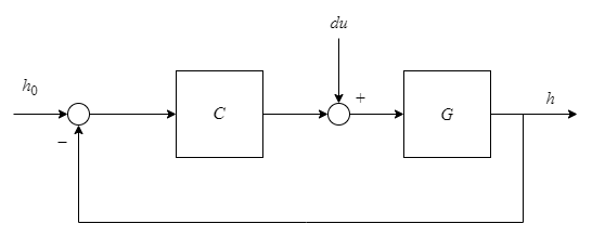
You must set the reference to to properly initialize the system and maintain it around = .
Create the model and discretize it.
hmin = 0.05;
hmax = 0.25;
h0 = (hmin+hmax)/2;
Ts = 0.01;
Glpv = lpvss("h",@fcnMaglev,0,0,h0);
Glpvd = c2d(Glpv,Ts,"tustin");
Sample the LPV model for three height values and tune a PID controller.
hpid = linspace(hmin,hmax,3);
[Ga,Goffset] = sample(Glpvd,[],hpid);
wc = 50;
Ka = pidtune(Ga,"pidf",wc);
Ka.Tf = 0.01;
Create the gain-scheduled PID controller.
Ka.SamplingGrid = struct("h",hpid);
Koffset = struct("y",{Goffset.u});
Clpv = ssInterpolant(ss(Ka),Koffset);
Create the closed-loop model.
CL = feedback(Glpvd*[1,Clpv],1,2,1);
CL.InputName = {'du';'href'};
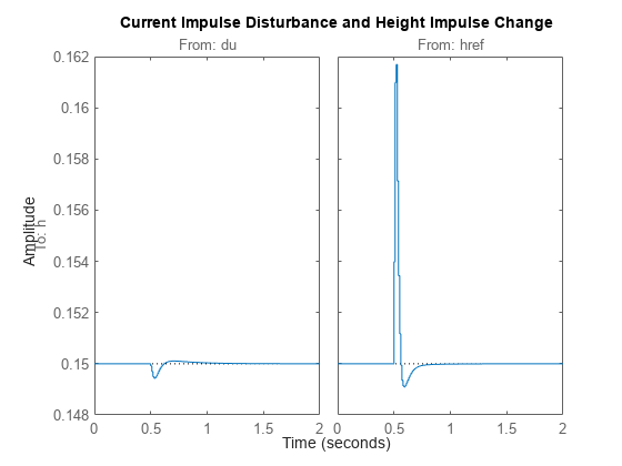
CL.OutputName = "h";Get steady-state current for = to size the disturbance
[~,~,~,~,~,~,~,u0] = Glpv.DataFunction(0,h0);
Response to impulse change in and .
t = 0:Ts:2;
pFcn = @(k,x,u) x(1);
Config = RespConfig(...
    InputOffset=[0;h0], ...
    Amplitude=0.2*[u0;h0]*Ts, ...
    Delay=0.5, ...
    InitialParameter=h0);
impulse(CL,t,pFcn,Config)
title("Current Impulse Disturbance and Height Impulse Change")
Input Arguments
Output Arguments
Limitations
The impulse response of a continuous system with nonzero D matrix is infinite at t = 0.
impulseignores this discontinuity and returns the lower continuity value Cb at t = 0.The
impulsecommand does not work on continuous-time models with internal delays. For such models, usepadeto approximate the time delay before computing the impulse response.The
impulsecommand does not support simulation along an implicit parameter trajectory for continuous-time LPV models.
Tips
When you need additional plot customization options, use
impulseplotinstead.To simulate system responses to arbitrary input signals, use
lsim.
Algorithms
Continuous-time LTI models are first converted to state-space form. The impulse response of a single-input state-space model
is equivalent to the following unforced response with initial state b.
To simulate this response, the system is discretized using zero-order hold on the inputs.
The sample time is chosen automatically based on the system dynamics, except when a time
vector t = T0:dt:Tf is supplied. Hence, dt is used as
sample time.
Version History
Introduced before R2006aSee Also
Linear System Analyzer | step | initial | lsim | pade | impulseplot
You can also select a web site from the following list:
Americas
- América Latina (Español)
- Canada (English)
- United States (English)
Europe
- Belgium (English)
- Denmark (English)
- Deutschland (Deutsch)
- España (Español)
- Finland (English)
- France (Français)
- Ireland (English)
- Italia (Italiano)
- Luxembourg (English)
- Netherlands (English)
- Norway (English)
- Österreich (Deutsch)
- Portugal (English)
- Sweden (English)
- Switzerland
- United Kingdom (English)